Geoelectrics
Theory
(text)
For further details, see script of lecture Angewandte Geophysik II from Georg Kaufmann.
Material properties
Electrical resistivity \(\rho_e\) [\(\Omega\)m].
Instrument(s)
GEOLOC GeoTom MK8E1000 RES/IP/SP: The Geotom from Geoloc is a processing unit to perform geoelectrical measurements in arbitrary geometry. It consists of the GEOTOM, the registration unit, and up to four cables with connections for steel electrodes, and steel electrodes. Additionally needed is a notebook, on which the GEOTOM software is installed. Connection between unit and notebook is via an USB cable.
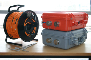
GeoTom MK8E1000 RES/IP/SP, photo Geoloc
Assembly
Important: Handle with extreme care!
In the field, lay out the profile line, possibly with survey tapes.
Unroll the cable drums along the profile. If more that one cable is used, position the processing unit in the center of the profile. Connect steel electrodes to the cable by first pushing the steel electrodes into the ground (no force!) and then clip them to the connector on the cable.
Our three cables have electrode positions every 5 meter. For shorter electrode distances, a measuring tape is needed to map the correct distances. If more than two cables are used, an extension cable is needed for the outer cable.
Connect the processing unit to ground by connecting a short cable to the green plug and an electrode (grounded).
Connect the processing unit to the notebook with the USB cable.
Configuration
Switch on the notebook.
Start the program
GeotomEand load a configuration file (the english version).Switch on the processing unit.
Field measurement
For every new line, first make a coupling test. Under
File->New, choose Coupling test, then a context window opens. Check electrode spacing, number of electrodes, and underoptionscheck the direction of each cable. The electrode positions are labelled on the cable, and you need to decide, where the first electrode is located, and if the cables are in normal or reverse position.Once the coupling test was successful, run a new measurement. Under
File->New, choose the layout (e.g. Wenner, Schlumberger, …). In the context window, check electrode spacing, number of electrodes, and underoptionscheck the direction of each cable.Start the measurement either with the traffic light button, or under (MISSING). If the Geotom unit is not switched on, the program will remind you.
Once the measurement is completed, save the data:
First, save the data in native format (
file->save).Second, export the data in Res2DInv format (
file->export).
Data download
Data are stored on the laptop and can be downloaded.
Post processing
Important:
Package Res2DInv is used for post processing.
As alterative, the pyGimli software is used for post processing.
From the field measurements, you should have saved the coupling file,
the native Geotom measurement file, and the exported measuring file. For
a profile named Campus_ERT03 this should be:
Campus_ERT03.ascCampus_ERT03.wenorCampus_ERT03.slmCampus_ERT03wen.datorCampus_ERT03slm.dat
For the latter two files, the first one indicates the Wenner setup, the second one the Schlumberger setup. Other setup configurations are possible.
The exported Res2DInv file looks like:
Rigole03
 3.00000
 1
  92
0
0
    0.000     3.000     90.54
    3.000     3.000     74.49
    6.000     3.000     87.19
...
    9.000    21.000     79.61
    0.000    24.000     73.20
0
0
first line is the profile name
second line the electrode spacing
third line indicates the type of ERT layout (1-Wenner, …)
fourth line the number of measurements
fifth and sixth line offsets
then the data section follows (profile distance, depth level, specific resistivity)
Georeferencing
We need to add coordinates and elevations for all electrodes to achieve a proper geo-referenced data file. This coordinate information needs to be added before we invert the ERT profile, as the topographical information influences the inversion.
See section on coordinate proesssing!
With coodinates, the Res2DInv formatted file looks like:
Rigole03
 3.00000
 1
  92
0
0
    0.000     3.000     90.54
    3.000     3.000     74.49
    6.000     3.000     87.19
...
    9.000    21.000     79.61
    0.000    24.000     73.20
2
25
  0.000 43.72
  3.000 43.85
  6.000 43.87
  9.000 43.94
 12.000 44.00
 15.000 43.97
 18.000 43.90
 21.000 43.93
 24.000 43.85
 27.000 43.88
 30.000 43.89
 33.000 43.92
 36.000 43.92
 39.000 43.88
 42.000 43.92
 45.000 43.94
 48.000 43.98
 51.000 43.90
 54.000 43.93
 57.000 44.08
 60.000 44.05
 63.000 44.04
 66.000 44.03
 69.000 44.04
 72.000 44.11
1
0
0
Now, the file Campus_ERT03.dat can be loaded
(File -> Read data file) into Res2DInv and inverted. For the
inversion, it is advisory to choose a robust inversion
(Inversion -> Selected robust inversion) and mark select YES to
all of the above options. Then start the inversion
(Inversion -> Least-squares inversion).
If you are satisfied with the result, display the inversion result
(Display -> Show inversion results). At the end, save the inverse
results to an ASCII file (File -> Save data in XYZ format), with the
option store as negative values.
