k-means Clustering

The k-means clustering is a popular unsupervised machine learning algorithm that groups data points into distinct clusters. As the name suggests, the algorithm divides a data set into a given number (k) of clusters, based on their individual arithmetic mean. In this introduction, we will explore how to use k-means in Python and provide an explanation of the algorithm.

To begin, let's define a function that will help us visualize the results. The function will create a scatter plot with different colors representing the clusters.

import matplotlib.pyplot as plt
import numpy as np
import pandas as pd
import seaborn as sns

def plot_clusters(data, cluster):
    sns.scatterplot(x='x', y='y', data=data, hue=cluster, palette='tab10')
    plt.title('k-means Clustering')
    plt.xlabel('Feature 1')
    plt.ylabel('Feature 2')

Now, let's generate some random toy data to demonstrate the k-means algorithm. We'll use a two-dimensional data set and plot it using the plot_clusters function.

rng = np.random.default_rng(seed=0)
data = pd.DataFrame({'x': rng.normal(size=35),
                     'y': rng.normal(size=35)})

# set a fixed cluster number for all points
plot_clusters(data, 0)

The data points are currently plotted with a single color, indicating that they haven't been clustered yet.

To apply the k-means algorithm, we'll use the KMeans function from the sklearn package in Python. First, we specify the algorithm by choosing the method to select the initial cluster centers, the number of clusters we want and the number of times the algorithm should run. Second, we run the algorithm on our data.

from sklearn.cluster import KMeans

kmeans = KMeans(init="random",
                n_clusters=4,
                n_init=1,
                random_state=0)
kmeans.fit(data)

KMeans(init='random', n_clusters=4, n_init=1, random_state=0)

After running the fit, we can access the assigned cluster for each data point using kmeans.labels_.

Let's update our plot to visualize the clusters obtained from k-means.

clusters = kmeans.labels_
plot_clusters(data, clusters)

The data points are colored based on the assigned clusters. The algorithm has separated the data into four distinct clusters.

Now, that we've seen how to apply the algorithm and visualize the resulting clusters, we want to explore the algorithm in depth.

The k-means algorithm

When clustering data, we aim for a high similarity of data points within each cluster and maximal dissimilarity between different clusters. The k-means algorithm achieves this by minimizing the sum of squared distances between points and their assigned centroid within each cluster. The corresponding optimization problem is $$\underset{\mathcal{C}}{\arg \min} \left( \sum_{i=1}^{k} \sum_{\boldsymbol{x}\in C_i}\| \boldsymbol{x} - \boldsymbol{\mu}_i \|^2\right),$$

with $\boldsymbol{x}\in \mathbb{R}^d$ where $d\in \mathbb{N}$ is the dimensionality of the data, $k\in \mathbb{N}$ the number of clusters, $\mathcal{C}=\{C_1,C_2, ... , C_k\}$ the set of clusters and $\boldsymbol{\mu}_i \in \mathbb{R}^d$ the mean (or centroid) of cluster $C_i$. $\|\cdot\|$ is usually the Euclidean norm, but based on the nature of the data or problem, other distance metrics can be used.

The algorithm can be broken down into five steps:

1. Choose the number of clusters k, e.g. k = 2.
2. Select k random points from the data set as initial centroids.
3. Assign each data point to its closest centroid.
4. Recompute the centroid (i.e. compute the mean) of each newly formed cluster.
5. Repeat step 3 and 4 until the iteration stops.

To demonstrate, how k-means works we will start from scratch and develop the algorithm step by step in the following. We start again with a set of randomly distributed, unclustered data points.

plot_clusters(data, 0)

Step 1: Choose number of clusters

For the algorithm itself, the first step is irrelevant, but it is certainly necessary to pass k , along with the data, to our function. Let's call our function k_means_clustering.

k = 4

def k_means_clustering(data, k):
    pass # we will fill this soon

Step 2: Initialize centroids

The initial centroids will be k randomly chosen data points from our data set.

def k_means_clustering(data, k):
    # select k centroids from the initial points
    centroids = data.sample(n=k, random_state=0).reset_index()
  
    return centroids

centroids = k_means_clustering(data, k)
plot_clusters(data, 0)
sns.scatterplot(x='x', y='y', data=centroids,
                s=100, marker='s', hue=[0, 1, 2, 3],
                palette=['#1f77b4', '#ff7f0e', '#2ca02c', '#d62728'],
                legend=False)
plt.show()

Step 3: Assign each data point to its closest centroid

So far, our function is capable of randomly selecting a given number of points. Now, we will form clusters by assigning each point to its closest centroid. Therefore, we compute the distances of all data points to each centroid and select the minimum, respectively. Usually, the Euclidean norm, commonly known as the Euclidean distance, serves as distance metric. However, based on the nature of the data or problem other distance metrics can also be used.

def k_means_clustering(data, k):
    # select k centroids from the initial points
    centroids = data.sample(n=k, random_state=0).reset_index()
    
    # compute distances (Euclidean norm)
    distances = pd.DataFrame()
    for cent in range(k):
        distances[cent] = np.sqrt((data['x']-centroids.at[cent, 'x'])**2
                                  + (data['y']-centroids.at[cent, 'y'])**2)

    # assign data to centroids
    cluster_assignment = distances.apply('idxmin', axis=1)
  
    return cluster_assignment, centroids

clusters, centroids = k_means_clustering(data, k)

plot_clusters(data, clusters)
sns.scatterplot(x='x', y='y', data=centroids,
                s=100, marker='s', hue=[0, 1, 2, 3],
                palette=['#1f77b4', '#ff7f0e', '#2ca02c', '#d62728'],
                legend=False)
plt.show()

Step 4: Recompute the centroid according to arithmetic mean

Now, that we have an initial clustering, we compute the arithmetic mean of each cluster to be the new centroid.

def k_means_clustering(data, k):
    # select k centroids from the initial points
    centroids = data.sample(n=k, random_state=0).reset_index()
    
    # compute distances (Euclidean norm)
    distances = pd.DataFrame()
    for cent in range(k):
        distances[cent] = np.sqrt((data['x']-centroids.at[cent, 'x'])**2
                                  + (data['y']-centroids.at[cent, 'y'])**2)

    # assign data to centroids
    cluster_assignments = distances.apply('idxmin', axis=1)
    
    # update centroids based on mean of the assigned data points
    new_centroids = pd.DataFrame(columns=['x', 'y'], index=range(k))
    for cent in range(k):
        new_centroids.iloc[cent] = pd.Series({'x': np.mean(data[cluster_assignments == cent].x),
                                              'y': np.mean(data[cluster_assignments == cent].y)})
  
    return cluster_assignments, new_centroids

clusters, centroids = k_means_clustering(data, k)

plot_clusters(data, clusters)
sns.scatterplot(x='x', y='y', data=centroids,
                s=100, marker='s', hue=[0, 1, 2, 3],
                palette=['#1f77b4', '#ff7f0e', '#2ca02c', '#d62728'],
                legend=False)
plt.show()

Step 5: Repeat step 3 and 4 until stop condition

Finally, we iterate step 3 and 4 until a stopping criterion is fulfilled. Possible stopping criteria are:

• Centroids of newly formed clusters do not change
• Points within one cluster remain the same
• Maximum number of iterations is reached

Here, we will stop the iteration when the centroids converge towards a fixed position.

def k_means_clustering(data, k):
    # select k centroids from the initial points
    centroids = data.sample(n=k, random_state=0).reset_index()
    
    # stopping criterion
    converged = False

    # iteration
    while not converged:
    
        # compute distances (Euclidean norm)
        distances = pd.DataFrame()
        for cent in range(k):
            distances[cent] = np.sqrt((data['x']-centroids.at[cent, 'x'])**2
                                      + (data['y']-centroids.at[cent, 'y'])**2)
        
        # assign data to centroids
        cluster_assignments = distances.apply('idxmin', axis=1)
    
        # update centroids based on mean of the assigned data points
        new_centroids = pd.DataFrame(columns=['x', 'y'], index=range(k))
        for cent in range(k):
            new_centroids.iloc[cent] = pd.Series({'x': np.mean(data[cluster_assignments == cent].x),
                                                  'y': np.mean(data[cluster_assignments == cent].y)})
        
        # Check for convergence
        if new_centroids.equals(centroids):
              converged = True
        else:
            centroids = new_centroids
  
    return cluster_assignments, new_centroids

clusters, centroids = k_means_clustering(data, k)

plot_clusters(data, clusters)
sns.scatterplot(x='x', y='y', data=centroids,
                s=100, marker='s', hue=[0, 1, 2, 3],
                palette=['#1f77b4', '#ff7f0e', '#2ca02c', '#d62728'],
                legend=False)
plt.show()

Properties

The k-means algorithm has some important properties:

• Limitations: It assumes that clusters have similar sizes and densities and is therefore limited to those cases. As we see in the following examples, k-means clustering solutions may not be suitable in situations where clusters are of varying sizes and densities.
  

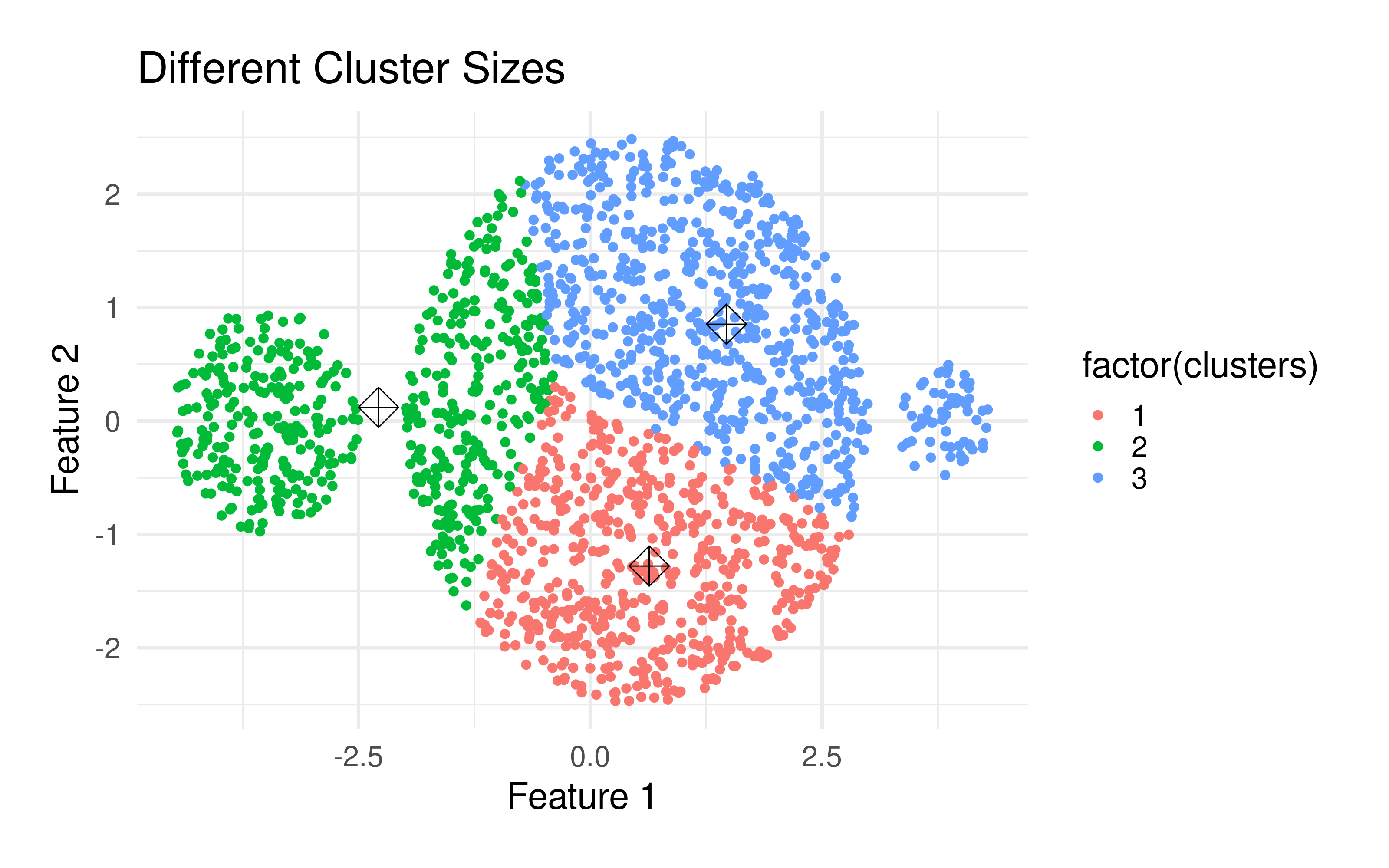
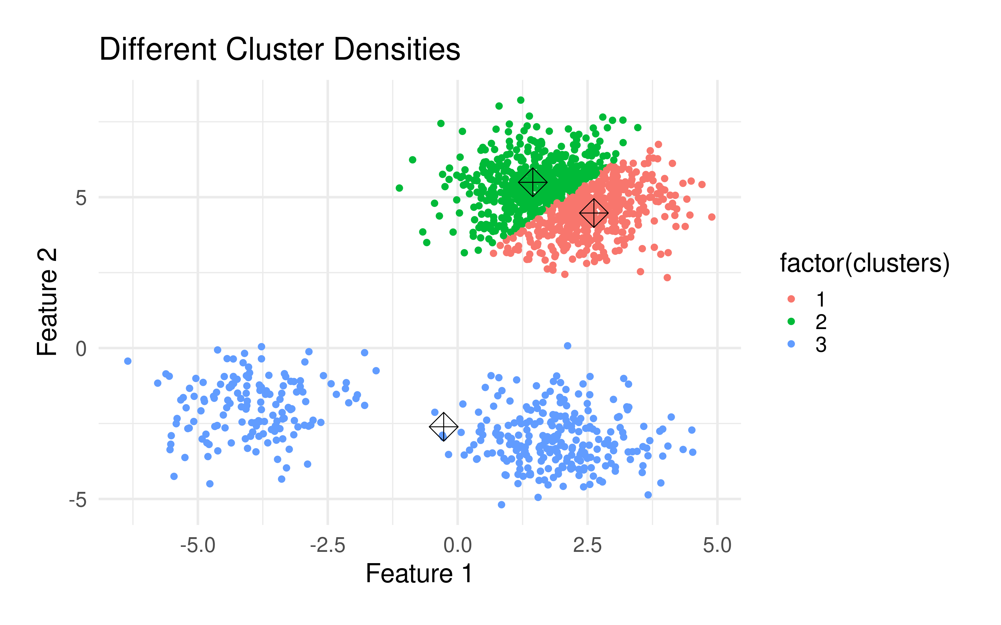
• Initialization: K-means requires specifying the number of clusters in advance. The selection of k significantly affects the final clustering result. But which number of clusters is optimal? Usually, when using this method, you want to divide the data set into a specific number of clusters. If you are not sure, there are several methods to determine the optimal number. Such are the Elbow method), which hierarchizes several runs with different k's, the Average silhouette method) and the Gap statistic method, among others.

Because of the randomness of the initial placement of centroids, running the algorithm several times will lead to different clustering solutions. To find the optimal clustering, multiple runs are recommended.

import urllib.request

fp = urllib.request.urlopen("https://userpage.fu-berlin.de/soga/soga-py/citation/citation_py.html")
mybytes = fp.read()

citation = mybytes.decode("utf8")
fp.close()

from IPython.display import display, HTML
display(HTML(citation))

---

Citation

The E-Learning project SOGA-Py was developed at the Department of Earth Sciences by Annette Rudolph, Joachim Krois and Kai Hartmann. You can reach us via mail by soga[at]zedat.fu-berlin.de.

You may use this project freely under the Creative Commons Attribution-ShareAlike 4.0 International License.

Please cite as follow: Rudolph, A., Krois, J., Hartmann, K. (2023): Statistics and Geodata Analysis using Python (SOGA-Py). Department of Earth Sciences, Freie Universitaet Berlin.