In this section we will learn how to read and process raster images and multiband raster images. We will process Landsat 8 imagery of the Berlin region downloaded from the U.S. Geological Survey (USGS) EarthExplorer on October, 14 2022. The observation data of the Landsat 8 scene we will work with is the August, 3 2022. You may easily access the data here.

# First, let's import the needed libraries.
import numpy as np
import matplotlib.pyplot as plt
import pandas as pd
import geopandas as gpd
import rasterio

from glob import glob

A tutorial on how to use the USGS EarthExplorer Website is given here. Note that downloading data products from the USGS might take some time and requires and account!

Once we downloaded the .tar folder containing our desired scene from the USGS EartExplorer we will untar it with the help of python. For the sake of this tutorial, you may download the Landsat scene here and put it in your respective directory.

import os
import tarfile

# create output folder
newFolder = "../data/LandsatScene_Berlin"

# check if folder exist already
if os.path.isdir(newFolder) == False:
    os.mkdir(newFolder)

# extract files
tar = tarfile.open("../data/LC08_L1TP_193023_20220803_20220806_02_T1.tar", "r:tar")
tar.extractall(newFolder)
tar.close()

You may want to check for he file size prior to loading the file. Processing large raster images can result in very long computing times.

filepath = "../data/LandsatScene_Berlin/LC08_L1TP_193023_20220803_20220806_02_T1_B4.TIF"
print(f"The file size is {os.path.getsize(filepath)/1e6} MB")

The file size is 94.067522 MB

When working with rasterdata of huge file sizes it can be very helpful to reduce the resolution for lower computation times. We will now plot a low-resolution overview of the Landsat 8 scene. Remember to set the no-data value to NaN for an improved colormap, since pixels outside of the scene are automatically set to "0". If you want to learn about this method, click here.

# acces raster as grid values as a numpy array and plot:
# https://geohackweek.github.io/raster/04-workingwithrasters/
with rasterio.open(filepath) as L8_src:
    oviews = L8_src.overviews(1)  # list of overviews from biggest to smallest
    oview = oviews[-1]  # smallest thumbnail
    print("Decimation factor= {}".format(oview))
    # NOTE this is using a 'decimated read' (http://rasterio.readthedocs.io/en/latest/topics/resampling.html)
    low_res = L8_src.read(
        1, out_shape=(1, int(L8_src.height // oview), int(L8_src.width // oview))
    )


plt.imshow(low_res, cmap="terrain")
plt.colorbar(label="reflectance * 1000")
plt.title("L8 2022-08-03 - Band 4")


plt.show()

Decimation factor= 64

EarthPy library is makes it very easy to work with spatial raster and vector data using open source tools. Especially when it comes to working with remotely sensed imagery, e.g. multiband raster images it is a nice addition to the rasterio package. EarthPy is also based on GeoPandas for the vector data while rasterio for the raster data. It also requires matplotlib for plotting operations. A nice tutorial about the earthpy package is given in the documentation.

Subsetting raster data

Another way to reduce the size of the raster data is to crop it to the area of interest. Here, we are only interested in the Berlin region. We will load a shape file covering Berlin, convert to the right crs, get the total_bounds of the Berlin shapefile and cut the window of the L8_band4 raster to size with the help of the EarthPy package.

Note: It is crucial to convert all geospatial data to the same coordinate reference system (crs)!

# Retrieve Federal States

import zipfile, requests, io

url = "https://daten.gdz.bkg.bund.de/produkte/vg/vg5000_0101/aktuell/vg5000_01-01.utm32s.shape.ebenen.zip"

r = requests.get(url)
z = zipfile.ZipFile(io.BytesIO(r.content))
z.extractall(path="../data")
germany_admin = gpd.read_file(
    "../data/vg5000_01-01.utm32s.shape.ebenen/vg5000_ebenen_0101/VG5000_LAN.shp"
)

# load shapefile of Berlin
berlin = germany_admin[germany_admin["GEN"] == "Berlin"]
berlin = berlin.to_crs("epsg:4326")

from rasterio.plot import plotting_extent

# open L8 band 4
with rasterio.open(filepath) as src:
    L8 = src.read(masked=True)[0]
    extent = rasterio.plot.plotting_extent(src)
    soap_profile = src.profile

# check for crs of landsat 8 image
setup_crs = src.crs
setup_crs

# convert to Landsat crs
berlin = berlin.to_crs(setup_crs)

# get total_bounds of berlin shapefile
xmin, ymin, xmax, ymax = berlin.total_bounds
xmin, ymin, xmax, ymax

(369991.8490680457, 5799545.725492317, 415748.2566591516, 5837135.521504402)

import earthpy as et
import earthpy.plot as ep
import earthpy.spatial as es

fig, ax = plt.subplots(figsize=(5, 5))
ep.plot_bands(
    L8,
    cmap="Greys",
    vmin=0,
    vmax=20000,
    extent=extent,
    ax=ax,
    cbar=True,
    title="L8 2022-08-03 - Band 4",
)
berlin.plot(ax=ax, alpha=0.9, color="red",)

<Axes: title={'center': 'L8 2022-08-03 - Band 4'}>

We use the crop_image function from earthpy.spatial to crop the raster layer to the total bounds of a shapefile. If you want to learn more about this method, you may click here.

with rasterio.open(filepath) as L8:
    L8_crop, L8_meta = es.crop_image(L8, berlin)

# Update the metadata to have the new shape (x and y and affine information)
L8_meta.update(
    {
        "driver": "GTiff",
        "height": L8_crop.shape[0],
        "width": L8_crop.shape[1],
        "transform": L8_meta["transform"],
    }
)

berlin_ext = [xmin, ymin, xmax, ymax]
bound_order = [0, 2, 1, 3]

berlin_ext = [berlin_ext[b] for b in bound_order]
berlin_ext, berlin.total_bounds

([369991.8490680457, 415748.2566591516, 5799545.725492317, 5837135.521504402],
 array([ 369991.84906805, 5799545.72549232,  415748.25665915,
        5837135.5215044 ]))

# mask the nodata and plot the newly cropped raster layer
L8_crop_ma = np.ma.masked_equal(L8_crop[0], -9999.0)

fig, ax = plt.subplots(figsize=(8, 8))
ep.plot_bands(
    L8_crop_ma,
    title="Landsat 8 - Band 4 \n Berlin August, 3 2022",
    cmap="Greys",
    vmin=0,
    vmax=20000,
    cbar=True,
    ax=ax,
)
plt.show()

---

RGB composites

As elaborated in the previous chapter, the landsat satellites carry multiple spectral sensors. Each of them comes with individuals properties for capturing light reflected at different wavelengths ranges. The reflectance at different wavelengths is stored as so-called bands for each Landsat scene. Remind yourself about the spectral properties of each Landsat 8 band in the previous section.

Spectral imaging describes the process of using multiple bands across the electromagnetic spectrum (EMS) for imaging. The human eye is able to capture the visual light (VIS) across three electromagnetic wavelength bands in the visible spectrum, red, green, and blue (RGB). Spectral imaging goes beyond the VIS, since wavelenghts across the EMS can be captured through different instruments.

Multispectral imaging captures a small number of spectral bands, typically three to roughly ten. The images are stored as so-called multiband raster images. They consist of multiple bands covering considered discrete ranges of wavelengths of the EMS. Therefore, a multi-spectral image is a collection (or stack) of bands of the same scene, each of them taken with a different sensor. Multispectral images can be visualized trough a RGB composite, where three bands or combined for one compositional images

E. g., a basic color image consists the three bands red (R), green (G), and blue (B). The composititon of the pixel brightness for each band (R,G, and B) creates the colors that we see in an image.

If you want to learn more about the Landsat band combinations for RGB composites, check out this blogpost.

EarthPy provides ready to use funcitonalities for processing multiband raster data. You may see the documentation of EarthPy, for a tutorial on how to create an RGB composite. We may easily use the EarthPy package for loading or raster data, since it integrates the rasterio functionality.

First, we need to list all band in the given directory, that we want to further process.

# Get list of bands and sort by ascending band number (2-7)
landsat_bands_data_path = glob(
    "../data/LandsatScene_Berlin/LC08_L1TP_193023_20220803_20220806_02_T1_B*[2-7]*.TIF"
)
landsat_bands_data_path

['../data/LandsatScene_Berlin\\LC08_L1TP_193023_20220803_20220806_02_T1_B2.TIF',
 '../data/LandsatScene_Berlin\\LC08_L1TP_193023_20220803_20220806_02_T1_B3.TIF',
 '../data/LandsatScene_Berlin\\LC08_L1TP_193023_20220803_20220806_02_T1_B4.TIF',
 '../data/LandsatScene_Berlin\\LC08_L1TP_193023_20220803_20220806_02_T1_B5.TIF',
 '../data/LandsatScene_Berlin\\LC08_L1TP_193023_20220803_20220806_02_T1_B6.TIF',
 '../data/LandsatScene_Berlin\\LC08_L1TP_193023_20220803_20220806_02_T1_B7.TIF']

The next crucial step is the stacking of the Landsat bands. We will use the earthpy.spatial.stack() and assign a value for empty raster cells (nodata).

# Create image stack and apply nodata value for Landsat
L8_stack, meta = es.stack(landsat_bands_data_path, nodata=-9999)

Now, we are ready to plot the RGB composite using the earthpy.plot.plot_rgb() function. Make sure to put your input bands on the right output channel (rgb argument. If you want to learn more about band combinations for Landsat 8, click here.

Note: The plot_rgb() input argument rgb takes the indices of the three bands to be plotted and not the band number itself! You have to check the right input indices in advance!

E.g. if the want to plot a RGB true color composite, we will have to check the indice of each band in the landsat_bands_data_path array. In this specific case we will put:

R = Red = Band 4 = Indice in landsat_bands_data_path = 2
G = Green = Band 3 = Indice in landsat_bands_data_path = 1
B = Blue = Band 2 = Indice in landsat_bands_data_path = 0

### Plot ####
fig, ax = plt.subplots(figsize=(6, 6))

# Plot RGB
# Red = Band 4, Green = Band 3, Blue = Band 2
ep.plot_rgb(
    L8_stack,
    rgb=(2, 1, 0),
    ax=ax,
    title="Landsat 8 RGB True Colors Image",
    stretch=True,
)
plt.show()

C:\Users\mceck\miniconda3\envs\rasterdata\lib\site-packages\numpy\lib\function_base.py:4691: UserWarning: Warning: 'partition' will ignore the 'mask' of the MaskedArray.
  arr.partition(

---

RGB composite of a cropped raster stack

If we just to look at a specific area of our raster stack, we need to crop all bands in advance, prior to stacking. The es.crop_all() function is an efficient way to crop all bands in an image quickly. The function will write out cropped rasters to a specified directory and return a list of file paths that can then be used with es.stack(). If you want to learn more about stacking, check out the EarthPy documentation on this.

Again, the first step will be listing all files we want to crop and stack. Then, we will create an output directory.

# Get list of bands and sort by ascending band number (1-7)
landsat_bands_data_path = glob(
    "../data/LandsatScene_Berlin/LC08_L1TP_193023_20220803_20220806_02_T1_B*[2-7].TIF"
)

# Create output directory and the output path
output_dir = "../data/LandsatScene_cropped"
# if path doesnt exist, built direcotry
if os.path.isdir(output_dir) == False:
    os.mkdir(output_dir)

Now, we are ready to crop all bands.

# crop to boundary of Berlin
band_paths_list = es.crop_all(
    landsat_bands_data_path, output_dir, berlin, overwrite=True
)

All of our desired bands are now cropped. We will create a new stack.

landsat_cropped_array, landsat_raster_profile = es.stack(band_paths_list, nodata=-9999)

crop_extent = plotting_extent(
    landsat_cropped_array[0], landsat_raster_profile["transform"]
)

First we will plot all monochromatic bands in the stack. Each band is stored as a grey scale image.

titles = ["Blue", "Green", "Red", "NIR", "SWIR 1", "SWIR 2"]
# sphinx_gallery_thumbnail_number = 1
ep.plot_bands(landsat_cropped_array, title=titles)

plt.tight_layout()
plt.show()

<Figure size 640x480 with 0 Axes>

Now, we are ready to plot the RGB true color composite using the earthpy.plot.plot_rgb() function by combining the R,G and B band.

### Plot ####
fig, ax = plt.subplots(figsize=(12, 6))
berlin.boundary.plot(ax=ax, color="red", zorder=10)
ep.plot_rgb(
    landsat_cropped_array,
    rgb=(2, 1, 0),
    ax=ax,
    stretch=True,
    extent=crop_extent,
    title="RGB True Color composite and Boundary Berlin \n August, 3 2022",
)
plt.show()

C:\Users\mceck\miniconda3\envs\rasterdata\lib\site-packages\numpy\lib\function_base.py:4691: UserWarning: Warning: 'partition' will ignore the 'mask' of the MaskedArray.
  arr.partition(

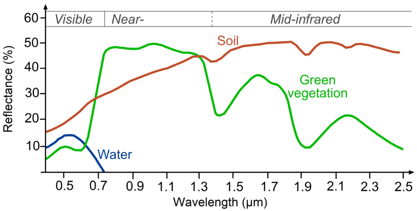
If we want to qualitatively observe other properties of our area of interest, we might also plot a different RGB composite. Land cover types come with different spectral characteristics, as they show different reflectance patterns across the EMS. E.g. Vegetation has a

Spectral signatures of specific land cover types, Source: Zanchetta 2017.

This Landsat 8 imagery was observed im summer on August, 3 2022, we might also look at the vegetation properties of the area at that time. Vegetation has a distinct pattern between the red band and the niR, the so-called red edge. Therefore, for the following composite we will use these two bands to highlight pixels with high vegetation density. For a Infrared composite we need the following spectralbands on the RGB channels:

R = Near-Infrared (nIR) = Band 5 = Indice in landsat_bands_data_path = 3
G = Red = Band 4 = Indice in landsat_bands_data_path = 2
B =  Green = Band 3 = Indice in landsat_bands_data_path = 1

Please note, that the band indices might change depending on your input directory call.

### Plot ####
fig, ax = plt.subplots(figsize=(12, 6))
berlin.boundary.plot(ax=ax, color="black", zorder=10)
ep.plot_rgb(
    landsat_cropped_array,
    rgb=(3, 2, 1),
    ax=ax,
    stretch=True,
    extent=crop_extent,
    title="RGB Infrared composite and Boundary Berlin \n August, 3 2022",
)
plt.show()

C:\Users\mceck\miniconda3\envs\rasterdata\lib\site-packages\numpy\lib\function_base.py:4691: UserWarning: Warning: 'partition' will ignore the 'mask' of the MaskedArray.
  arr.partition(

Areas in red indicate a higher vegetation density.

Now, we saw how to read and process multiband raster images and crop them to the area of interest. In the next section we will deal with raster calculations.

---

Citation

The E-Learning project SOGA-Py was developed at the Department of Earth Sciences by Annette Rudolph, Joachim Krois and Kai Hartmann. You can reach us via mail by soga[at]zedat.fu-berlin.de.

You may use this project freely under the Creative Commons Attribution-ShareAlike 4.0 International License.

Please cite as follow: Rudolph, A., Krois, J., Hartmann, K. (2023): Statistics and Geodata Analysis using Python (SOGA-Py). Department of Earth Sciences, Freie Universitaet Berlin.