A symmetric moving average $(m_t)$ for the observation $x_t$ is given by
$$m_t = \sum_{j=-k}^k a_jx_{t-j}\text{,}$$where $a_j = a_{-j}$ and $\sum_{j=-k}^ka_j = 1$.
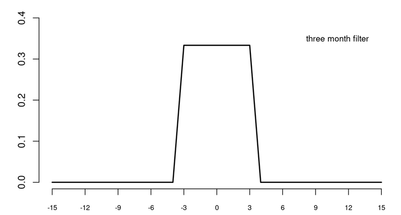
Consider a monthly time series. A 3-month low pass filter can be written in mathematical notation as
$$m_t = \frac{1}{3}(x_{t-1}+x_t+x_{t+1})$$# First, let's import the needed libraries.
import pandas as pd
import matplotlib.pyplot as plt
import numpy as np
from datetime import datetime
The simple moving average is the unweighted mean of the previous data points (3 in the example above). The selection of M (moving window) depends on the degree of smoothing desired. Increasing the value of M improves the smoothing, but at the same time decreases the accuracy.
A symmetric 3-month low pass filter works according to the following principle:

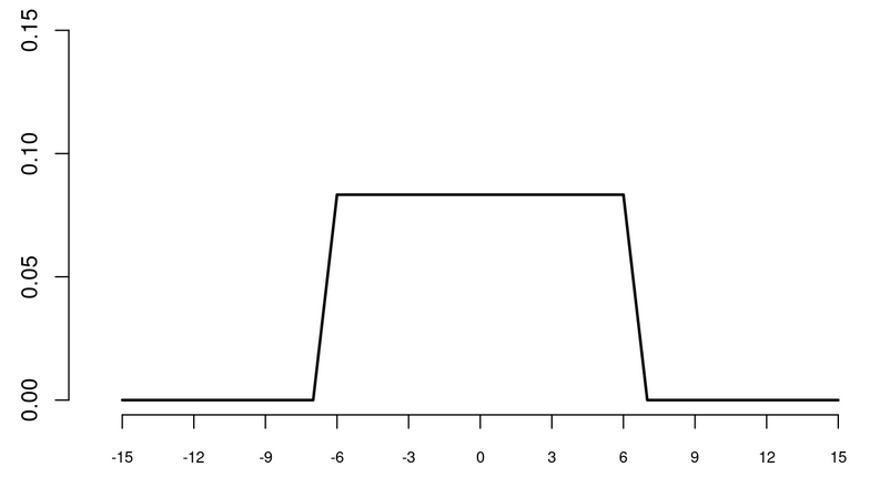
In contrast, a symmetric one-year filter is specified by:

In Python calculating the moving average is fairly easy accomplished by using the pandas.Series.rolling() function. On the resulting windows, we can perform calculations using a statistical function. The size of the window is specified by the argument window.
Read more about the functionality of the method here.
Let us build three low pass filters:
# read the Earth Surface Temperature data t_global.json, processed in the previous section
# read the data from .json file
t_global = pd.read_json(
    "http://userpage.fu-berlin.de/soga/soga-py/300/307000_time_series/t_global.json"
)
t_global["Date"] = pd.to_datetime(t_global["Date"], format="%Y-%m-%d", errors="coerce")

# subset
temp_global = t_global.set_index("Date")["1850-01-01":"2021-12-31"][
    "Monthly Anomaly_global"
]
temp_global
Date
1850-01-01   -1.886
1850-02-01   -0.149
1850-03-01   -0.536
1850-04-01   -1.130
1850-05-01   -1.358
              ...
2021-08-01    1.198
2021-09-01    1.275
2021-10-01    1.577
2021-11-01    1.307
2021-12-01    1.351
Name: Monthly Anomaly_global, Length: 2064, dtype: float64
Rolling window operations are an important transformation for time series data. Rolling windows overlap and "roll" along at the same frequency as the data, so the transformed time series is at the same frequency as the original time series. The window size is the same as the frequency in the data. E.g. here we are dealing with monthly aggregated data, this means a one-year rolling window has the window size 12.
By default, all data points within a window are equally weighted in the aggregation, but this can be changed by specifying window types such as Gaussian, triangular, and others. We will stick to the standard equally weighted window here.
We use the center=True argument to label each window at its midpoint, so the rolling windows are:
# Compute the centered 1 year rolling mean
temp_global_f1 = temp_global.rolling(min_periods=1, window=12, center=True).mean()


# Compute the centered 5 year rolling mean
temp_global_f5 = temp_global.rolling(min_periods=1, window=12 * 5, center=True).mean()

# Compute the centered 10 year rolling mean
temp_global_f10 = temp_global.rolling(min_periods=1, window=12 * 10, center=True).mean()
## plotting
fig, ax = plt.subplots(figsize=(18, 6))

ax.plot(
    temp_global,
    linestyle="-",
    linewidth=0.3,
    label="Monthly Data",
    color="grey",
)

ax.plot(
    temp_global_f1,
    marker="o",
    markersize=1,
    linestyle="-",
    label="one-year filter",
)

ax.plot(
    temp_global_f5, marker=".", markersize=1, linestyle="-", label="five-year filter"
)


ax.plot(
    temp_global_f10, marker=".", markersize=1, linestyle="-", label="five-year filter"
)

ax.legend()
<matplotlib.legend.Legend at 0x1aaaeb4ab00>
The rolling() function is quite flexible, hence it is straightforward to define a custom filter.
Exercise: Design a custom symmetric seven-year filter for a monthly time series that gives full weight to the measurement year, three-quarters weight to adjacent year, half weight to years two removed, and quarter weight to years three removed.
Unfortunately, there is no built-in function if we want to use custom weights on the data. But we can apply a weighted moving average with a corresponding rolling window (make use of the apply() function).
## Your code here...
# construct the pattern
weights = np.array([0.25, 0.5, 0.75, 1, 0.75, 0.5, 0.25])
Let us apply our custom symmetric seven-year filter and plot the result.
temp_global_weigths = temp_global.rolling(7).apply(
    lambda x: np.average(x, weights=weights)
)

## plotting
fig, ax = plt.subplots(figsize=(18, 6))

ax.plot(
    temp_global,
    linestyle="-",
    linewidth=0.3,
    label="Monthly Data",
    color="grey",
)

ax.plot(
    temp_global_weigths,
    marker="o",
    markersize=1,
    linestyle="-",
    label="custom seven-year filter",
)

ax.legend()
<matplotlib.legend.Legend at 0x1aaaec5f430>
With the functionality of the rolling() we may for example analyse the time series of the earth surface temperature anomalies with respect to the question if the variability in the monthly mean temperature changes within a window of 30 years.
Therefore, we first define our reference period. Let us say our reference period is the 30-year period from 1986 to 2021.
# reference period
ref_period = t_global.set_index("Date")["1986-01-01":"2021-12-31"][
    "Monthly Anomaly_global"
]
# reference period standard deviation
ref_period_sd = ref_period.std()
ref_period_sd
0.44274650376216834
In the next step we apply the rolling() function in combination with the mean() function.
The rolling() function has no additional argument for applying a non-overlapping sliding window. We got a few options for adding an non-overlapping window.
For one, we could compute the usual rolling() function and then skip every $n^{th}$ row (here: n = 30).
w = 30 * 12

## not overlapping rolling window:
std_30years = temp_global.rolling(min_periods=0, window=w).apply(lambda x: np.std(x))[
    w - 1 :: w
]
std_30years
Date
1879-12-01    0.516120
1909-12-01    0.378498
1939-12-01    0.348118
1969-12-01    0.308923
1999-12-01    0.393496
Name: Monthly Anomaly_global, dtype: float64
fig, ax = plt.subplots(figsize=(18, 6))
std_30years.plot(kind="bar", ax=ax, color="lightgrey", edgecolor="grey")

# generate more informative labeling

ax.set_xticklabels(
    ["1850-1879", "1880-1909", "1910-1939", "1940-1969", "1970-1999"],
    rotation=0,
)

plt.axhline(
    y=ref_period_sd,
    linewidth=1,
    linestyle="dashed",
    color="r",
    label="stdev reference period (1986-2015)",
)

plt.title(
    "Standard deviation of mean monthly temperature anomalies for \na 30-year non-overlapping sliding window"
)
plt.legend()
plt.show()
Another option is the resample function, where we set the 30-year-period ("30Y") and then calculate the standard deviation.
std_30years = temp_global.resample("30Y").std()
std_30years = std_30years[:-1]  # drop row for 2030
std_30years = std_30years.iloc[1:]  # drop entry for >1850
std_30years
Date
1880-12-31    0.505551
1910-12-31    0.376124
1940-12-31    0.348937
1970-12-31    0.309233
2000-12-31    0.397152
Freq: 30A-DEC, Name: Monthly Anomaly_global, dtype: float64
fig, ax = plt.subplots(figsize=(18, 6))
std_30years.plot(kind="bar", ax=ax, color="lightgrey", edgecolor="grey")

# generate more informative labeling

ax.set_xticklabels(
    ["1850-1879", "1880-1909", "1910-1939", "1940-1969", "1970-1999"],
    rotation=0,
)

plt.axhline(
    y=ref_period_sd,
    linewidth=1,
    linestyle="dashed",
    color="r",
    label="stdev reference period (1986-2015)",
)

plt.title(
    "Standard deviation of mean monthly temperature anomalies for \na 30-year non-overlapping sliding window"
)
plt.legend()
plt.show()
See how both methods yield in the same result!
We got a nice bar plot. The plot suggest that the variability in mean monthly temperatures during the reference period 1986-2015 was higher, compared to the 30-year time periods of 1880-1909, 1910-1939, 1940-1969, 1970-1999. However, during the 30-year periods of 1850-1879 the variability of mean monthly temperatures appears to be even higher than during the reference period of 1986-2015.
Now we can take this analysis even a step further.
Exercise: Repeat the analysis from above, this time however, evaluate the standard deviation of mean monthly temperature anomalies for a 30-year period for each year in the time series (overlapping sliding window).
The code is nearly the same as the code from above.
## Your code here...
w = 30 * 12

## overlapping rolling window:
std_30years = temp_global.rolling(min_periods=w, window=w).apply(lambda x: np.std(x))
# # plotting
fig, ax = plt.subplots(figsize=(18, 6))


ax.plot(
    std_30years,
    linestyle="-",
    linewidth=1,
    label="stdev",
    color="black",
)

plt.axhline(
    y=ref_period_sd,
    linewidth=1,
    linestyle="dashed",
    color="r",
    label="stdev reference period (1986-2015)",
)

plt.title(
    "Standard deviation of mean monthly temperature anomalies for 30-year non-overlapping sliding window"
)


plt.legend()
plt.show()
Citation
The E-Learning project SOGA-Py was developed at the Department of Earth Sciences by Annette Rudolph, Joachim Krois and Kai Hartmann. You can reach us via mail by soga[at]zedat.fu-berlin.de.

Please cite as follow: Rudolph, A., Krois, J., Hartmann, K. (2023): Statistics and Geodata Analysis using Python (SOGA-Py). Department of Earth Sciences, Freie Universitaet Berlin.