There are nearly unlimited reasons for scale transformation. Here we are focusing on the following

  • Scale homogeneity
  • Algebraic constraints on positive feature scales
  • Skewness, symmetry and normality
  • Compositional data sets
  • Double constraint feature scales

Scale inhomogeneity

When measuring the temperature, we have the choice between different units: Kelvin [K], Celsius [°C] or Fahrenheit [°F]. Whereas Kelvin has an absolute orign of 0°K, the other two have arbitrary zero pints. A simple shift of -273.15 links the Celsius and Kelvin scale. In order to build physically meaningful statistical models such transformation have to be performed first.

Further examples are different currencies, molar weight and mass weight percentages of e.g. chemical compositions or length, area and volume units in meter, yard, inches etc..

Such type of transformations can be described by linear relations as $$ y=b*x + a $$ The constant a is the shift or translation value and b the slope or stretching factor. In the following chapter, we will call these linear relations as scaling (translation & stretching). Example Transformation from Celsius )($x$) to Fahrenheit: $$ \underbrace{y}_{[°F]} = \underbrace{1.8* x + 32}_{[°F]} \, .$$

Algebraic constraints on limited feature scales

Most real-world variables can only be positive (e.g. $\mathbb{R_+}$ or $]0,+\infty]$ or are limited to an interval ($]a,b[_\mathbb{R_+}$). Exceeding these boundaries by algebraic operations such as (+,-,*,/) leads to useless or meaning less results.

Example On the scale of positive real numbers $\mathbb{R_+}$ multiplication and the inverse operation division can not leave the set of positive real numbers. Thus, the positive real numbers together with the multiplication, denoted by $(\mathbb{R_+},*)$, form a commutative group with 1 as neutral element. In contrast, the set of positive real numbers together with the addition $(\mathbb{R_+},+)$ has neither inverse elements nor a neutral element. Thus, addition and subtraction can not be unlimited performed. But a log-transformation of any variable $$x\in\mathbb{R_+}: x\to x'=\log(x)$$ opens the scale to $x'\to\mathbb{R}$ and transforms the neutral element of $(\mathbb{R_+},\cdot)$ given by 1 to the neutral element of $(\mathbb{R},+)$, given by 0! The field of $(\mathbb{R},+,\cdot)$ provides nearly unlimited operations for statistical purposes (except e.g. $\sqrt{-1}$ or $\frac{1}{0}$).

The inverse transformation powering $$x'\to x=e^{x'}$$

reverse the log-transformation back to the positive reel scale.

Skewness, symmetry and normality

Let us look on the following example on a data set of measured dissolved Mg:

DissolvedMG

We obtain:

  • Min: 0.11
  • 1st Qu.: 0.63
  • Median: 1.05
  • arithmetic Mean: 1.42
  • 3rd Qu.: 1.74
  • Max.: 15.13

Compared with the median, the arithmetic mean appears as a bad estimate of central tendency for our heavy skewed data. Let us try the geometric mean as measure of central tendency:

  • geom. Mean: 1.04

Obviously the geometric mean seems to be a far better estimate for the central tendency. One reason for right skewed distributions can be the Hoelder inequality $\bar{x}_{geo}\leq \bar{x}_{arith}$, but is not sufficient as explanation. Let us recall the geometric mean: $$ \bar{x}_{geo}=\sqrt[n]{\prod_{i=1}^N x_i}=\prod_{i=1}^N x_i^{\frac{1}{n}}= x_1^{\frac{1}{n}}\cdot x_2^{\frac{1}{n}}\cdots x_n^{\frac{1}{n}}$$ The main apparent difference between these two means is the operator: sum for arithmetic mean and product for the geometric mean. Thus, the arithmetic mean recommend for an additive or distance scale and the geometric mean for a ratio scale approach. In our case, we are dealing with a variable clearly hosted on the $\mathbb{R}_+$-scale where only multiplication is unlimited allowed.

But we often need an arithmetic mean for further statistical parameters: e.g.

  • standard deviation
  • skewness
  • covariance
  • correlation
  • regression
  • etc.

To solve this problem, we can apply the logarithm to the geometric mean: \begin{align} log(\bar{x}_{geo}) & =log(x_1^{\frac{1}{n}}\cdot x_2^{\frac{1}{n}}\cdots x_n^{\frac{1}{n}})= \\ & =\frac{1}{n}log(x_1)+\frac{1}{n}log(x_2)+\cdots+\frac{1}{n}log(x_N)= \\ & =\frac{1}{n}\sum_{i=1}^{N}{log(x_i)}={\overline{log(x_i)}}_{arith} \end{align}

!!! The logarithm of the geometric mean is the arithmetic mean of the logarithms!!!

Applying logarithm on our Mg-data yield the following distribution:

DissolvedMG-on-log-scale

Using the log-transformation kill two birds with one stone:

  1. We transform our data on the feature scale $\mathbb{R}$ with nearly unlimited operations

concerning differences and ratios! 2. We are getting a less skewed nearly normal distribution, where symmetric confidence intervals are becoming meaningful.

Checking for normality using the Shapiro test confirm that the distribution is normal!

Now, regarding this transformed data set, we are allowed to apply all concepts based on standard deviations and we can calucate the means and confidence intervals in the usual way!

After doing these statistics, do not forget to transform the results back onto the original feature scale. As explained above, we can do this applying the exponential function.

Comparison:

Calculate moments and interval the "wrong" way not using the transformations and compare the output with the transformed data:

DissolvedMg-means

Here, the green lines showing geometric mean including CI and 2-sigma-intervals after back transformation (the robust way). The same in red represents the meaningless mean and interval margins. We call it "meaningless" at least due to the negative concentration suggested by the lower 2-sigma-margin of the arithmetic mean.

Magnification of the CI's exhibit the difference in both CI's:

Drawing

On the original feature scale, the robust CI's are skew as the random model.

Other transformations to gain normality / symmetry but do not solve algebraic constraints:

  • square-root-transformation
  • reciprocal
  • $asin$-transformation
  • $asin-sqrt$-transformation

Important:

In our example above, we kept the problem of upper scale limit. No concentration can be larger than 100% or 1000g/kg, etc. . Here, the upper limit is far below 1000g/liter due to a chemical saturation limit. However, nearly all observable measures are physical or ecological (economical, demographical etc.) limited, at least on earth. We will come back to this problem after explaining the statistical, algebraic and geometric problem of compositional constraints.

Compositional contraints

If the level of investigation of compositional data with classical tools moves from a descriptive phase to the application of statistical tests, erroneous evaluation of the formulated hypothesis maybe the result, a serious point when environmental questions are the matter of debate. from A. Buccianti, 2013. Is compositional data analysis a way to see beyond the illusuion?

Compositions are sets of variables which values sum up to a constant:

  • dissolved cations and anions in a liquid
  • frequencies of population groups (e.g. employees, jobless people, etc.)
  • role allocation of a person during a time span in behavioral sciences
  • nutrition content for food declaration
  • many, many more ...

Due to the compositional nature of such variable, they can neither be independent nor normal.

*A simple example:*

Let us generate a 3-part random composition by defining 2 random variables and a remainder to the total. All three parts should be independent.

A B C
Min. 0.4925 0.4783 40.63
1st Qu. 7.9098 11.8154 52.27
Median 21.3940 17.6066 62.03
Arithm. mean 18.4264 17.9454 63.63
3rd Qu. 27.4527 25.2677 75.83
Max 31.5422 32.4978 86.17

All three parts should be independent.

matrix

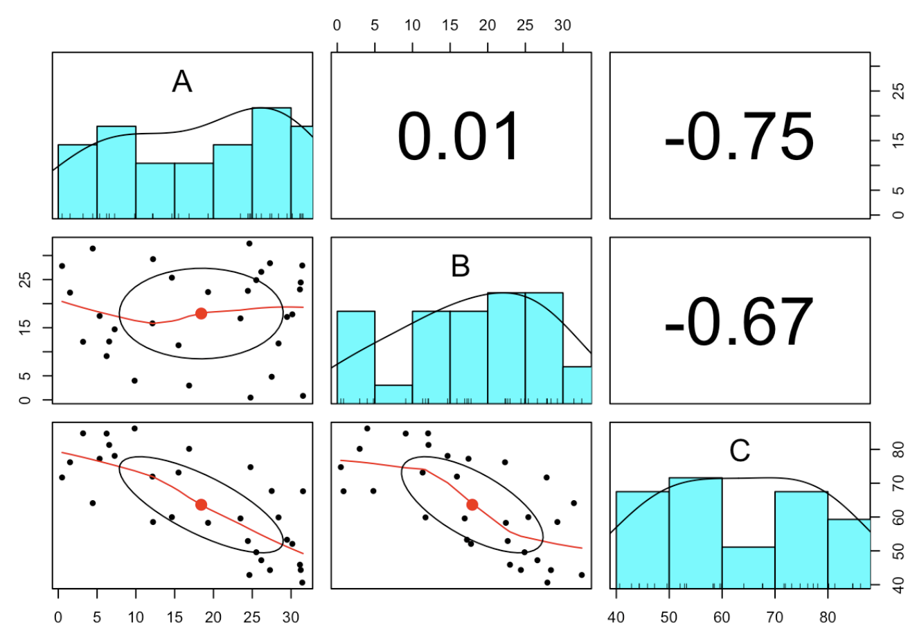
As we see, both random variables are correlated with the remainder. Imagine, we are measuring another part and extent the composition by variable D. Hereby, we re-generate C as random and close all 4 parts to 100%:

matrix

If closing a set of independent uniform random variable to 100%, none of them stay uniform anymore. They are loosing any symmetry and possible initial normality! Furthermore, beside A and B all correlations are negative again.

Testing for significance of the Pearson correlation coefficient leads to the following result:

50% of possible pairs of random variable are showing up with significance correlation!

What does this imply beside obvious spurious correlations?

We can interpret the correlation coefficient as normalized cosine of the angle between the deviation vectors to the mean $$\mathbf{x}_{d}=(x_i-\bar{x},i=1,\cdots,n)$$

and

$$ \mathbf{y}_{d}=(y_i-\bar{y},i=1,\cdots,n)$$

The cosine of the angle between two vectors is calculated by the scalar product divided to the product of both norm:

$$\cos \measuredangle (\mathbf{x}, \mathbf{y})=\frac{<\mathbf{x}, \mathbf{y}>}{\parallel \mathbf{x} \parallel \cdot \parallel \mathbf{y} \parallel }= \frac {\sum{x_i\cdot y_i }}{\sqrt{x_i^2}\cdot \sqrt{y_i^2}} $$

Setting $\mathbf{x} =\mathbf{x}-\overline{\mathbf{x}}$ and $\mathbf{y} =\mathbf{y}-\overline{\mathbf{y}}$, we are getting the scalar product as nominator for the covariance term and the product of the norms as standard deviation terms.

Thus, in compositions the deviations vectors as bases are oblique by nature and consequently non-euclidean!

Hence, statistical methods using distances and angles (ratios) as optimization parameters can not be applied on pure compositions. Such methods are e.g.:

  • (ML-)regression and correlation, GLM, PCA, LDA, ANN
  • SVM, KNN, k-Means
  • most hypotheses tests, etc.

Whereas, this problem is well known since Karl Pearson published the problem of spurious correlation in compositional data 1897 more than 100 years ago Felix Chayes suggest the use of ratios instead of portions: $$ a,b \in ]0,1[_{\mathbb{R}}\to \frac{a}{b}\in \mathbb{R_+} $$ One of the remaining disadvantage was now the question about nominator and denominator, because of the often huge difference between a/b and b/a. Another problem was still the limit to the positive reel feature scale.

In 1981, the Scottish statistician John Aitchison solved the problem introducing the log-ratios: $$ \log \frac{a}{b}=-\log \frac{b}{a}\in\mathbb R\, .$$ Thus, changing nominator and denominator just change the sign of the log-ratio but not the absolute value implies symmetry again (cf. paragraph above) In his Book The statistical analysis of composional data, 1986 introduced

  1. Additive log-ratio (alr) transformation is the logarithm of the ratio of each variable divided by a selected variable of the composition. Alr applied on a D-dimensional composition results in a D-1-dimensional variable space over the field $(\mathbb{R},+,\cdot)$. Unfortunately, beside a asymmetry in the parts, alr is not isometric. Thus, distances and angles are not consistence between simplex and the resulting D-1 dimensional subspace of $\mathbb{R}^D$.
  2. Centered log-ratio (clr) transformation is the logarithm of the ratio of each value divided through the geometric mean of all parts of the corresponding observation. The clr transformation is symmetric with respect to the compositional parts and keeps the same number of components as the number of parts in the composition. Due to the problem that orthogonal references in that subspace are not obtained in a straightforward manner, Egozcue et al. 2003 introduced:
  3. Isometric log-ratio (ilr) transformation is isometric and provides an orthonormal basis. Thus, distances and angles are independent from the sub-composition (symmetric in all parts of the sub-composition) comparable between the Aitchison simplex and the D-dimensional reel space.

However, PCA or SVD-analysis on a clr-transformed simplex provides similar properties Egozcue et al. 2003.

Double constrained feature spaces

There is a certain relation to the compositional constraint if we face double bounded feature spaces. Let us imagine a variable $\mathbf{x}=(x_i\in ]l,u[_\mathbb R,i=1,\cdots,m)$ within a constrained interval [a,b]$\subset \mathbb R$. The absolute value is obviously of minor interest compared with the relative position between l and u. A first step should be a linear min-max-transformation wit min=l and max=u:

$$ x \to x' =\frac{x-l}{u-l} \in\ ]0,1[\ \in \ {\mathbb R}_+ $$

Now, x' divides the interval into two parts: 1. the distance to the left (=x) and 2. the distance to the right (1-x). Both sum up to 1 and are therefore related to a 2-dimensional composition. Applying an alr-transformation to our variable, we are getting a symmetric feature scale: $$ x'\to x''=\log(\frac{x'}{1-x'})\in \mathbb R$$ This so-called logistic transformation enable application of algebraic operation over the base field $\mathbb R$.

Feature scales and machine learning approaches

As shown above, normalization, scaling, standardization and transformations are crucial requirements for reliable and robust application of statistical methods beyond simple data description for getting meaningful results. Especially application of complex machine learning algorithms for exploration of multivariate data patterns it often becomes likely to get entrapped for violation of important preconditions. Hereby, it can be the violation of scale homogeneity using gradient descent related optimization technics or non-euclidean feature space for distance or angle related technics as well as simple violation of algebraic constraints.

A brief overview of common risk concerning serious pitfall is provided by Minkyung Kang in his data science blog:

ML Models sensitive to feature scale

  • Algorithms that use gradient descent as an optimization technique
    • Linear Regression
    • Neural Networks
  • Distance-based algorithms
    • Support Vector Machines
    • KNN
    • K-means clustering
  • Algorithms using directions of maximized variances
    • PCA / SVD
    • LDA

ML models not sensitive to feature scale

  • Tree-based algorithms
    • Decision Tree
    • Random Forest
    • Gradient Boosted Trees

Citation

The E-Learning project SOGA-Py was developed at the Department of Earth Sciences by Annette Rudolph, Joachim Krois and Kai Hartmann. You can reach us via mail by soga[at]zedat.fu-berlin.de.

Creative Commons License
You may use this project freely under the Creative Commons Attribution-ShareAlike 4.0 International License.

Please cite as follow: Rudolph, A., Krois, J., Hartmann, K. (2023): Statistics and Geodata Analysis using Python (SOGA-Py). Department of Earth Sciences, Freie Universitaet Berlin.