Logistic regression analysis belongs to the class of [generalized linear models] (https://en.wikipedia.org/wiki/Generalized_linear_model). We apply a $L_2$-regularized logistic regression model, which we have explained in the introductory sections on logistic regression and regularization methods.
Suppose the response variable takes value in $G=\text{{0,1}}$. Denote $y_i=I(g_i=1)$. The model
$$P(G=1|X=x)+\frac{e^{\beta_0+\beta^{T}x}}{1+e^{\beta_0+\beta^{T}x}}$$can be written in the following form:
$$\log\frac{P(G=1|X=x)}{P(G=0|X=x)}=\beta_0+\beta^{T}x,$$the so-called logistic or log-odds transformation.
$$\min_{\substack{(\beta_0\beta)\in\mathbb{R}^{p+1}}}- \begin{bmatrix} \frac{1}{N}\displaystyle\sum_{i=1}^{N}y_i(\beta_0+x_i^T\beta)-\log(1+e^{\beta_0+x_i^T\beta}) \end{bmatrix}+\lambda[(1-\alpha)||\beta||_2^2/2+\alpha||\beta||_1].$$We use functionality of the sklearn
package to apply the regularized logistic regression model.
The LogisticRegressionCV()
function provides the $L_2$-regularized logistic regression model.
It takes the following arguments:
In previous sections we prepared the response vectors and the model matrices for the training and
test sets (y_train
, y_test
, X_train
, X_test
, X_train_PC3
, X_test_PC3
, and pca_PC3
).
Let us load all the data we need into our workspace.
# import packages
import folium
from matplotlib import pyplot as plt
import numpy as np
import pandas as pd
from sklearn.linear_model import LogisticRegressionCV
from sklearn.metrics import accuracy_score, cohen_kappa_score
# load model input data from previous section
y_train = pd.read_feather("https://userpage.fu-berlin.de/soga/data/py-data/y_train.feather").set_index("index")
y_test = pd.read_feather("https://userpage.fu-berlin.de/soga/data/py-data/y_test.feather").set_index("index")
X_train = pd.read_feather("https://userpage.fu-berlin.de/soga/data/py-data/X_train.feather").set_index("index")
X_test = pd.read_feather("https://userpage.fu-berlin.de/soga/data/py-data/X_test.feather").set_index("index")
X_train_PC3 = pd.read_feather("https://userpage.fu-berlin.de/soga/data/py-data/train_set_PC3.feather").set_index("index")
X_test_PC3 = pd.read_feather("https://userpage.fu-berlin.de/soga/data/py-data/test_set_PC3.feather").set_index("index")
HOT_DAY_train = pd.read_feather("https://userpage.fu-berlin.de/soga/data/py-data/HOT_DAY_train.feather").set_index("index")
HOT_DAY_test = pd.read_feather("https://userpage.fu-berlin.de/soga/data/py-data/HOT_DAY_test.feather").set_index("index")
pca_PC3 = pd.read_feather("https://userpage.fu-berlin.de/soga/data/py-data/pca_PC3.feather")
dwd_data = pd.read_feather("https://userpage.fu-berlin.de/soga/data/py-data/dwd_data.feather").set_index("index")
The general procedure is as follows:
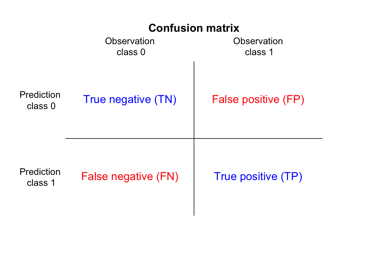
We evaluate the model performance by calculating the model accuracy, the confusion matrix and Cohen’s kappa. The confusion matrix is a specific table that visualizes the performance of a predictive model. Each column of the matrix represents the instances in a actual class while each row represents the instances in an predicted class (or sometimes vice versa).
Cohen’s kappa coefficient, $κ$, is a statistic which measures inter-rater agreement for categorical items. It takes a value of $κ=0$ if the items agreement is due to chance. A value of $κ=1$ indicates a perfect model fit.
The definition of $κ$ is:
$$\kappa=\frac{p_0-p_e}{1-p_e},$$where $p_0$ is the relative observed agreement (identical to accuracy), and $p_e$ is the hypothetical probability of chance agreement, using the observed data to calculate the probabilities of each observer randomly saying each category.
In the baseline model we predict the response variable HOT_DAY
by including all 15 features in
the data set. We use the $L_2$-regularized logistic regression model
(ridge regression:
alpha = 0
) provided by the sklearn
package. In particular we apply the LinearRegressionCV
class, which performs by default
cross-validation) on
the data set and evaluates the model performance.
# baseline model, binomial, logistic, rigde regression
m_log_baseline = LogisticRegressionCV(
penalty='l2', # L2 regularization
solver='lbfgs', # optimization algorithm
Cs=100, # values of the regularization parameter C to try
cv=10, # number of folds in cross-validation
scoring='accuracy', # scoring metric
random_state=0, # seed
max_iter=10000, # maximum number of iterations
n_jobs=-1, # number of parallel processes
refit=True, # refit the best model with the entire dataset
multi_class='ovr', # one-vs-rest
class_weight='balanced' # rebalance the data set
).fit(X_train, y_train.values.ravel())
Now we plot the relation between the misclassification error and the regularization parameter $λ$.
# plot misclassification error vs. lambda
plt.plot(m_log_baseline.Cs_, np.mean(m_log_baseline.scores_[1], axis=0))
plt.axvline(m_log_baseline.C_[0], c='k', ls='--')
plt.axvline(m_log_baseline.C_[0] * 0.1, c='k', ls=':')
plt.xscale('log')
plt.xlabel('lambda')
plt.ylabel('misclassification error')
plt.grid()
plt.show()
The plot shows that the misclassification error increases with $λ$. The dotted vertical lines indicate the value of $λ$ that gives the minimum mean cross-validated error and the largest value of $λ$ such that the error is within 1 standard error of the minimum.
# minimum lambda
m_log_baseline.C_
array([1.09749877])
# lambda within 1 standard error of the minimum
m_log_baseline.C_[0] * 0.1
0.10974987654930568
Finally, we use the test data set, X_test
, and the best $λ$ to predict the response vector
y_test
.
# prediction for the test set
m_log_baseline_pred = m_log_baseline.predict(X_test)
# prediction results
m_log_baseline_pred
array([1, 1, 1, 0, 1, 1, 1, 1, 1, 1, 1, 1, 1, 1, 1, 1, 1, 1, 1, 1, 1, 1, 1, 1, 1, 1, 0, 1, 1, 1, 1, 1, 1, 1, 1, 1, 1, 1, 1, 0, 1, 1, 1, 1, 1, 1, 0, 1, 1, 1, 1, 1, 1, 0, 1, 0, 1, 1, 1, 1, 0, 1, 0, 1, 1, 1, 1, 1, 0, 1, 0, 1, 1, 1, 1, 0, 1, 1, 1, 0, 1, 1, 0, 1, 1, 1, 1, 1, 1, 1, 1, 1, 1, 1, 1, 0, 0, 1, 1, 1, 1, 1, 1, 1, 1, 1, 1, 1, 1, 1, 1, 1, 1, 1, 1, 1, 1, 1, 1, 0, 0, 0, 1, 1, 1, 1, 1, 1, 1, 0, 1, 1, 1, 1, 1, 1, 1, 1, 1, 1, 1, 1, 0, 0, 0, 1, 1, 1, 1, 1, 1, 0, 1, 1, 1, 1, 0])
Now we have a look at the confusion matrix and the model accuracy. Specifically we look the accuracy and Cohen’s kappa.
# confusion matrix
cm = pd.crosstab(
pd.Series(y_test.values.ravel(), name="Actual"),
pd.Series(m_log_baseline_pred, name="Predicted"),
)
cm
Predicted | 0 | 1 |
---|---|---|
Actual | ||
0 | 20 | 0 |
1 | 4 | 133 |
# accuracy
accuracy_score(y_test.values.ravel(), m_log_baseline_pred)
0.9745222929936306
# Cohen's kappa
cohen_kappa_score(y_test.values.ravel(), m_log_baseline_pred)
0.8944182918628111
# Calculate the accuracy benchmark
dwd_data["HOT_DAY"].sum()/len(dwd_data["HOT_DAY"])
0.8639798488664987
The model performs very good. We perform better than our accuracy benchmark of $0.86$. The two model metrics, accuracy and Cohen's kappa are $0.97$ and $0.89$, respectively. In terms of classification accuracy we count $20$ true negative and $133$ true positive classifications. In contrast we only misclassified $4$ observations ($4$ false negatives and $0$ false positives).
Now we build a $L_2$-regularized logistic regression model to predict the response variable
HOT_DAY
by including just the first three principal components scores. As in the previous section,
we compute the confusion matrix, the model accuracy and Cohen’s kappa for the test set to evaluate
the goodness of fit of the model.
# build the model
m_log_PC3 = LogisticRegressionCV(
penalty="l2", solver="lbfgs", max_iter=10000, random_state=0
).fit(X_train_PC3, y_train.values.ravel())
# prediction for the test set
# we use the learned model and the new data
# We look for the smallest lambda
m_log_PC3_pred = m_log_PC3.predict(X_test_PC3)
# prediction results
m_log_PC3_pred
array([1, 1, 1, 0, 1, 1, 1, 1, 1, 1, 1, 1, 1, 1, 1, 1, 1, 1, 1, 1, 1, 1, 1, 1, 1, 1, 1, 1, 1, 1, 1, 1, 1, 1, 1, 1, 1, 1, 1, 1, 1, 1, 1, 1, 1, 1, 0, 1, 1, 1, 1, 1, 1, 1, 1, 1, 1, 1, 1, 1, 0, 1, 0, 1, 1, 1, 1, 1, 0, 1, 0, 1, 1, 1, 1, 0, 1, 1, 1, 0, 1, 1, 0, 1, 1, 1, 1, 1, 1, 1, 1, 1, 1, 1, 1, 0, 0, 1, 1, 1, 1, 1, 1, 1, 1, 1, 1, 1, 1, 1, 1, 1, 1, 1, 1, 1, 1, 1, 1, 0, 1, 0, 1, 1, 1, 1, 1, 1, 1, 0, 1, 1, 1, 1, 1, 1, 1, 1, 1, 1, 1, 1, 0, 1, 0, 1, 1, 1, 1, 1, 1, 0, 1, 1, 1, 1, 1])
# confusion matrix
cm = pd.crosstab(
pd.Series(y_test.values.ravel(), name="Actual"),
pd.Series(m_log_PC3_pred, name="Predicted"),
)
cm
Predicted | 0 | 1 |
---|---|---|
Actual | ||
0 | 14 | 6 |
1 | 3 | 134 |
# accuracy
accuracy_score(y_test.values.ravel(), m_log_PC3_pred)
0.9426751592356688
# Cohen's kappa
cohen_kappa_score(y_test.values.ravel(), m_log_PC3_pred)
0.7245077013062975
The model performs very good compared the baseline model. The PC3 model accuracy is higher than our accuracy benchmark of $0.86$. The two model metrics, accuracy and Cohen's kappa are $0.975$ and $0.725$ , respectively. We count $14$ true negative and $134$ true positive classifications. In contrast we only misclassified $9$ observations ($3$ false negatives and $6$ false positives).
Please note that we projected a 15-dimensional data set onto a 3-dimensional feature space, and still the model performance is remarkable.
Again, we use the folium
package to visualize the results on a map.
Let's first use our model m_log_PC3 to predict the occurrence of hot days at a particular weather station. Let us visualize the classification results of the PC3 model on a map.
# predict the occurrence of hot days at a particular weather station
m_log_PC3_full = m_log_PC3.predict(pca_PC3)
# add a new column called "Classification" to the data set
# "FN" for false negativ,
# "TN" for true negativ,
# "FP" for false positive and
# "TP" for true positive
# assign prediction vector to data set
dwd_data["Classification"] = m_log_PC3_full
# assign "FN" to all observations that are false negative
dwd_data.loc[
(dwd_data["Classification"] == 0) & (dwd_data["HOT_DAY"] == 1), "Classification"
] = "FN"
# assign "TN" to all observations that are true negative
dwd_data.loc[
(dwd_data["Classification"] == 0) & (dwd_data["HOT_DAY"] == 0), "Classification"
] = "TN"
# assign "FP" to all observations that are false positive
dwd_data.loc[
(dwd_data["Classification"] == 1) & (dwd_data["HOT_DAY"] == 0), "Classification"
] = "FP"
# assign "TP" to all observations that are true positive
dwd_data.loc[
(dwd_data["Classification"] == 1) & (dwd_data["HOT_DAY"] == 1), "Classification"
] = "TP"
# create a map
m = folium.Map(
location=[51.3, 10.5],
zoom_start=7,
tiles="cartodbpositron",
width="100%",
height="100%",
)
# add a tile layer to the map
folium.TileLayer("cartodbpositron").add_to(m)
# add a layer control panel to the map
folium.LayerControl().add_to(m)
# add a marker for each station
for i in range(len(dwd_data)):
if dwd_data.iloc[i]["Classification"] == "TP":
color = "green"
tooltip = "True Positive"
elif dwd_data.iloc[i]["Classification"] == "TN":
color = "blue"
tooltip = "True Negative"
elif dwd_data.iloc[i]["Classification"] == "FP":
color = "black"
tooltip = "False Positive"
elif dwd_data.iloc[i]["Classification"] == "FN":
color = "red"
tooltip = "False Negative"
else:
raise ValueError("Unexpected Classification value")
folium.Circle(
location=[dwd_data.iloc[i]["LAT"], dwd_data.iloc[i]["LON"]],
color=color,
tooltip=tooltip,
fill=True,
radius=1000,
).add_to(m)
# show the map
m
The map shows an interesting pattern. First of all we realize that the data set is quite imbalanced, as there are a lot more positives than negatives. We see that the negatives (weather stations that did not record a hot day so far) are clustered. One cluster is located in the Alpine region and the Alpine foothills. Another cluster is found in the Central German Uplands, and another cluster is observed at the coastal regions of Germany. Though, it is very interesting, that the classification algorithm correctly predicted all observations in the southern part of Germany. In the central parts of Germany the algorithm sometimes failed to correctly predict positives, as well as negatives. However, one pattern is very striking. In the coastal regions of Northern Germany the logistic regression model performed, in general, quite well, expect for those weather stations located in the federal state of Schleswig-Holstein. In this particular coastal region nearly all class predictions turn out to be wrong. This is an interesting result, which needs more thoroughly investigation.
Citation
The E-Learning project SOGA-Py was developed at the Department of Earth Sciences by Annette Rudolph, Joachim Krois and Kai Hartmann. You can reach us via mail by soga[at]zedat.fu-berlin.de.
Please cite as follow: Rudolph, A., Krois, J., Hartmann, K. (2023): Statistics and Geodata Analysis using Python (SOGA-Py). Department of Earth Sciences, Freie Universitaet Berlin.