The linear model is given by the equation
$$y = \alpha + \beta x + \epsilon$$where $\alpha$ is the intercept, $\beta$ is the regression coefficient and $\epsilon$ the error term. The best regression line is found by applying the ordinary least squares method, which minimizes the sum of squares error (SSE). This means minimizing the squared difference of the measured response variable $y$ and the model prediction $\hat y$, which is given by
$$SSE = \sum_{i = 1}^{n} \epsilon_{i}^{2} = \sum_{i = 1}^{n} (y - \hat y)^{2}$$Refer to the section on linear regression for more details on the linear model.
However, no matter what, we must acknowledge that we build our models, in this case, our linear regression model, on observation data. Hence, the data originates from a population whose corresponding statistical properties are generally unknown to us. Thus, by taking measurements, each observation represents a manifestation of the population denoted by the term random variable.
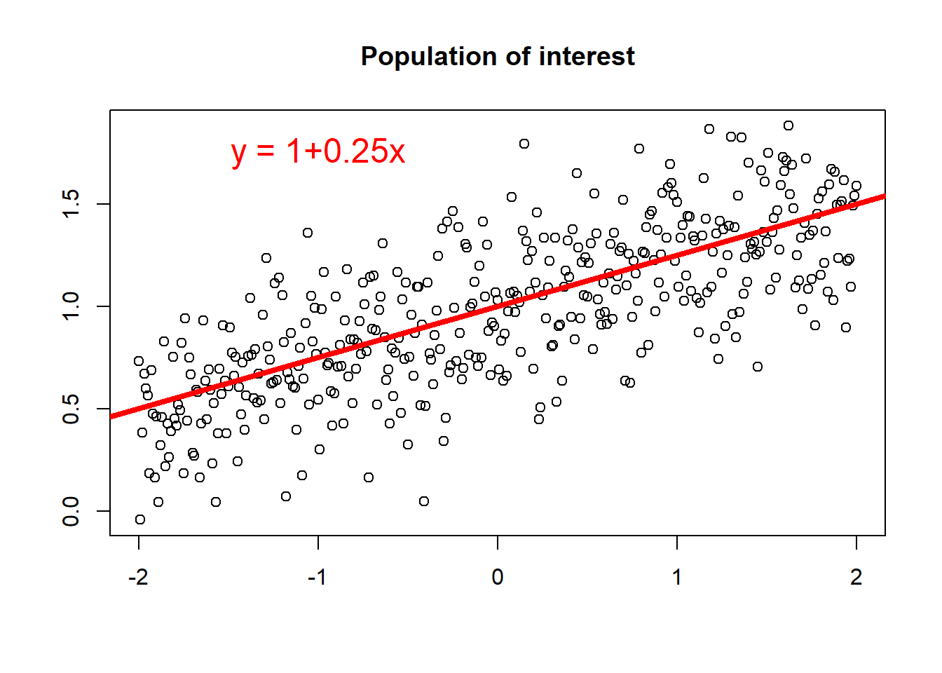
Let us consider the example shown in the figure below. In this example, the population parameters are known. Thus, we may build a linear regression model of $y = \alpha + \beta x = 1 + 0.25x$.
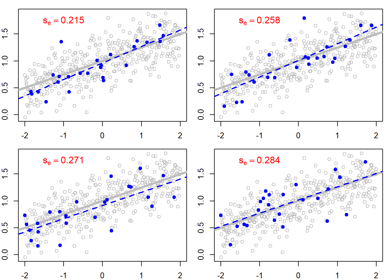
However, let's now take a random sample of the population and build a linear model based on the sample data. The sample regression line will be different from the population regression line. For the figure below, we take four random samples with a size of 25 (blue dots). We immediately see that the sample regression line (blue dashed line) differs from the population regression line (grey line). In order to account for that variability, which is due to the random sampling process, a statistic is calculated by applying the equation
$$s_{e} = \sqrt {\frac {SSE} {n - 2} }$$where $SSE$ corresponds to the sum of squares error and $n$ corresponds to the sample size. The statistic, $s_{e}$, is denoted as standard error of the estimate $(s_{e})$ or the residual standard error.
As seen above, the sample regression line varies from one sample to another and is, therefore, a random variable. Its distribution is called the sampling distribution of the slope of the regression line.
