In this section, we discuss hypothesis tests for two population standard deviations. In other words, we discuss methods of inference for the standard deviations of one variable from two different populations. These methods are based on the $F$-distribution, named in honour of Sir Ronald Aylmer Fisher.

The $F$-distribution is a right-skewed probability density distribution with two shape parameters, $v_{1}$ and $v_{2}$, called the degrees of freedom for the numerator ($v_{1}$) and the degrees of freedom for the denominator ($v_{2}$).

$$ df = (v_{1}, v_{2})$$

As for any other density curve, the area under the curve of the $ F$ distribution corresponds to probabilities. The area under the curve and, thus, the probability for any given interval and given $df$ is computed with software. Alternatively, one may look them up in a table. In those tables, generally, the degrees of freedom for the numerator ($v_{1}$) are displayed along the top, whereas the degrees of freedom for the denominator ($v_{2}$) is displayed in the outside column on the left.

In order to perform a hypothesis test for two population standard deviations, the value corresponding to a specified area under a $F$-curve is calculated.

Given $\alpha$, where $\alpha$ corresponds to a probability between 0 and 1, $F_{\alpha}$ denotes the value having an area $\alpha$ to its right under a $ F$ curve.

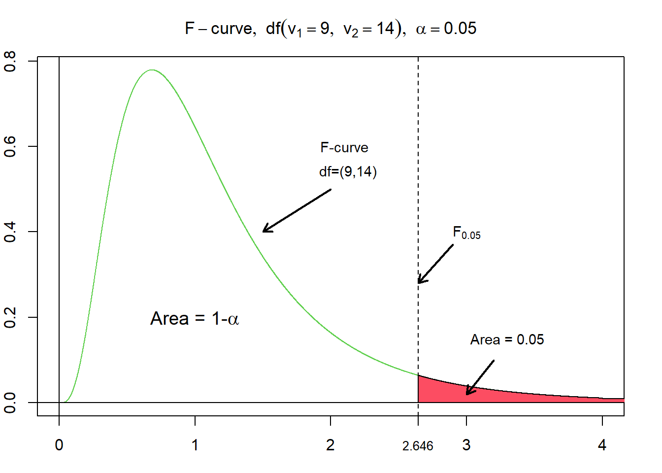
The figure above illustrates the probability density function of a F distribution with the degrees of freedom of 9 and 14. Additionally, the rejection and non-rejection areas regarding a right-tailed hypothesis test are added to a significance level of 95 %, respectively, with an alpha level of 5%. The corresponding, critical value, of $F_{0.05}$ for $df = (9,14)$ evaluates to $\approx 2.6458$.

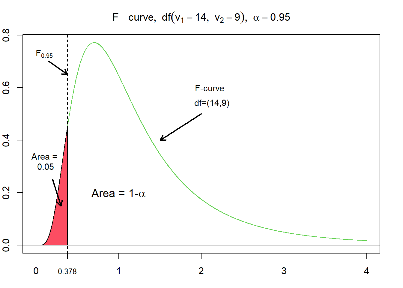
One interesting property of $F$-curves is the reciprocal property. This means, that for a $F$-curve with $df = (v_{1}, v_{2})$, the $F$-value having the area $\alpha$ to its left equals the reciprocal of the $F$-value having the area $\alpha$ to its right for an $F$-curve with $df = (v_{2}, v_{1})$ (Weiss, 2010). Adopted to the example from above, where $F_{0.05}$ for $df=(9,14)$ evaluates to $\approx 2.6458$, this means that $F_{0.95}$ for $df=(14,9)$ evaluates to $\frac {1} {2.6458} = 0.378$.

Interval Estimation of $\sigma_{1} - \sigma_{2}$

The $100(1 - \alpha)\ \%$ confidence interval for $\sigma$ is

$$\frac {1} {\sqrt {F_{\alpha /2} } } \times \frac {s_{1}} {s_{2}} \le \sigma \le \frac {1} {\sqrt {F_{1 - \alpha /2} } } \times \frac {s_{1}} {s_{2}} \text{,} $$

where $s_1$ and $s_2$ are the sample standard deviations.

Two Standard Deviations $F$-test

The hypothesis-testing procedure for two standard deviations is called two standard deviations $F$-test. Hypothesis testing for two population standard deviations follows the same step-wise procedure as for other hypothesis tests:

---

1. State the null hypothesis $H_{0}$ and alternative hypothesis $H_{A}$.
2. Decide on the significance level, $\alpha$.
3. Compute the value of the test statistic.
4. Determine the p-value.
5. If $p \le \alpha$, reject $H_{0}$; otherwise, do not reject $H_{0}$.
6. Interpret the result of the hypothesis test.

---

The test statistic for a hypothesis test for a normally distributed variable and for independent samples of sizes $n_{1}$ and $n_{2}$ is given by

$$F = \frac {s_{1}^{2} / \sigma_{1}^{2}} {s_{2}^{2} / \sigma_{2}^{2}} \text{,} $$

with $df = (n_{1} - 1,\; n_{2} - 1)$.

If $H_{0}: \sigma_{1} = \sigma_{2}$ is true, then the equation simplifies to

$$F = \frac {s_{1}^{2}} {s_{2}^{2}} \text{.} $$

Two Standard Deviations $F$-test: An example

In order to get some hands-on experience, we apply the two standard deviations $F$-test in an exercise. For this, we load the students data set. You may download the students.csv file here and import it from your local file system, or you load it directly as a web resource. In either case, you import the data set to python as pandas dataframe object by using the read_csv method:

import pandas as pd
import numpy as np

students = pd.read_csv("https://userpage.fu-berlin.de/soga/data/raw-data/students.csv")

Note: Make sure the numpy, pandas and scipy packages are part of your mamba environment!

The students data set consists of 8239 rows, each representing a particular student, and 16 columns, each corresponding to a variable/feature related to that particular student. These self-explaining variables are:

• stud.id
• name
• gender
• age
• height
• weight
• religion
• nc.score
• semester
• major
• minor
• score1
• score2
• online.tutorial
• graduated
• salary

In order to showcase the two standard deviations $F$-test, we examine once again the height variable in the students data set. We want to investigate if the standard deviation of the height of female students ($\sigma_{1}$) is statistically different from the standard deviation of the height of male students ($\sigma_{2}$).

Data preparation

We start with data preparation.

• We subset the data set based on the variable gender.
• We sample 25 female students and 25 male students.
• We calculate the standard deviations of female's and male's height as the variable of interest (height in cm) for assigning them the variables sample_std_females and sample_std_males.

n = 25

females_sample_height = students.loc[students.gender == "Female"].sample(n, random_state = 8)["height"]
males_sample_height = students.loc[students.gender == "Male"].sample(n, random_state = 8)["height"]

sample_std_females = np.std(females_sample_height, ddof = 1)
sample_std_males = np.std(males_sample_height, ddof = 1)

sample_std_females

7.397522107661006

sample_std_males

8.722002828097073

Further, we check the normality assumption by plotting a Q-Q plot. You can quickly generate a well-looking QQ-Plot in Python over the probplot() function provided over the stats module within the scipy package.

Note: Ensure matplotlib are installed in your mamba environment!

import matplotlib.pyplot as plt
import scipy.stats as stats

plt.figure(figsize=(12,5))

ax = plt.subplot(1, 2, 1)
qq = stats.probplot(females_sample_height, dist="norm", plot = plt)
ax.set_title("Q-Q plot for heights of\n sampled female students")
ax.set_ylabel("Sample quantiles")

ax = plt.subplot(1, 2, 2)
qq = stats.probplot(males_sample_height, dist="norm", plot = plt)
ax.set_title("Q-Q plot for heights of\n sampled male students")
ax.set_ylabel("Sample quantiles")

Text(0, 0.5, 'Sample quantiles')

The data of both samples falls roughly onto a straight line. Based on the graphical evaluation approach we conclude that the data is normally distributed.

Hypothesis testing

In order to conduct the two standard deviations $F$-test we follow the step-wise implementation procedure for hypothesis testing.

Step 1: State the null hypothesis $H_{0}$ and alternative hypothesis $H_{A}$

The null hypothesis states that the standard deviation of the height of female students ($\sigma_{1}$) equals the standard deviation of the height of male students ($\sigma_{2}$):

$$H_{0}: \quad \sigma_{1} = \sigma_{2}$$

Alternative hypothesis:

$$H_{A}: \quad \sigma_{1} \ne \sigma_{2}$$

This formulation results in a two-sided hypothesis test.

---

Step 2: Decide on the significance level, $\alpha$

$$\alpha = 0.05$$

alpha = 0.05

---

Step 3 and 4: Compute the value of the test statistic and the p-value

For illustration purposes we manually compute the test statistic in Python manually. Recall the equation for the test statistic from above:

$$F = \frac {s_{1}^{2}} {s_{2}^{2}}$$

F_statistic = (sample_std_males**2) / (sample_std_females ** 2)
F_statistic

1.3901443625510146

The numerical value of the test statistic is $\approx 1.390144$.

In order to calculate the p-value, we apply the f.cdf() function derived by the scipy package over the stats module to calculate the probability of occurrence for the test statistic based on the $F$ distribution. To do so, we also need the degrees of freedom. Recall how to calculate the degrees of freedom:

$$df = (n_{1} - 1, n_{2} - 1)$$

Note: Ensure scipy are installed in your mamba environment!

from scipy.stats import f

df_1 = df_2 = n - 1

p_value = f.cdf(F_statistic, df_1, df_2)

p_value

0.7872008348344762

$p = 0.78720083$

---

Step 5: If $p \le \alpha$, reject $H_{0}$; otherwise, do not reject $H_{0}$

# reject H0?

p_value < alpha

False

The p-value is greater than the specified significance level of 0.05; we do not reject $H_{0}$. The test results are statistically significant at the 5 % level and do not provide sufficient evidence against the null hypothesis.

---

Step 6: Interpret the result of the hypothesis test

At the 5 % significance level the data does not provide sufficient evidence to conclude, that the standard deviations of the heights of female and male students differ significantly from each other.

Hypothesis testing in Python with scipy

We just completed a two standard deviations $F$ test in Python manually. OK, we learned a lot, but now we use the power of Python's package universe, namely the scipy package, to perform a two standard deviations using just one line of code! Unfortunately, there is no pre-written implementation of an F-test. However, scipy provides two alternatives to perform a two standard deviations test. You can choose between the Bartlett’s test using the bartlett() function and the Levene test using the levene(). Both functions are available over the stats module within the scipy package. We will show the usage of both functions to reproduce the same test results as above. Additional information regarding the function's usage can be derived directly from the function's documentation of scipy.

Note: Since the metodological approach of the Bartlett’s test and the Levene test differ from the approach used by the $F$-Test the pvalues will be differently. Nevertheless, we shall observe similar test decisions regarding $H{0}$ and $H_{A}$.

Perform the Bartlett’s variances test

from scipy import stats

test_result = stats.bartlett(females_sample_height,
                             males_sample_height)

test_result

BartlettResult(statistic=0.6349065302325954, pvalue=0.42556125740617146)

The bartlett() function returns an object, which provides the teststatic as well as the corresponding p-value of the test result. Those values can be retrieved over the following properties:

• <object>.statistic holds the actual teststatic and represents the empirical test value.
• <object>.pvalue represents the p-value of the performed significance test.

Consequently, the teststatistic is retrieved over:

test_result.statistic

0.6349065302325954

The p-value is retrieved over:

test_result.pvalue

0.42556125740617146

Perform the Levene variances test

from scipy import stats

test_result = stats.levene(females_sample_height,
                           males_sample_height)

test_result

LeveneResult(statistic=0.8055230228687669, pvalue=0.3739269932367949)

The teststatistical values of interest can again be retrieved over the returned object:

print("Teststatistic = {}".format(round(test_result.statistic, 5)))
print("p-value = {}".format(round(test_result.pvalue, 5)))

Teststatistic = 0.80552
p-value = 0.37393

Excellent, both test results support our evidence from above that we can not reject $H_{0}$ based on a significance level of 95 %!

---

Citation

The E-Learning project SOGA-Py was developed at the Department of Earth Sciences by Annette Rudolph, Joachim Krois and Kai Hartmann. You can reach us via mail by soga[at]zedat.fu-berlin.de.

You may use this project freely under the Creative Commons Attribution-ShareAlike 4.0 International License.

Please cite as follow: Rudolph, A., Krois, J., Hartmann, K. (2023): Statistics and Geodata Analysis using Python (SOGA-Py). Department of Earth Sciences, Freie Universitaet Berlin.