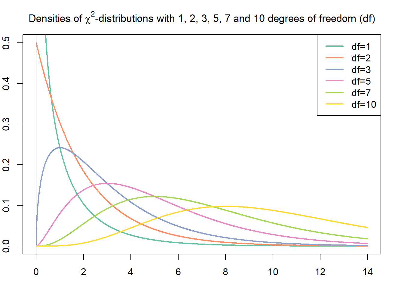
Inferences for one population standard deviation are based on the *chi-square ($\chi^2$) distribution*. A $\chi^{2}$-distribution is a right-skewed probability density curve. The shape of the $\chi^{2}$-curve is determined by its degrees of freedom $(df)$.

In order to perform a hypothesis test for one population standard deviation, we relate a $\chi^{2}$-value to a specified area under a $\chi^{2}$-curve. Either we consult a $\chi^{2}$-table to look up that value, or we use Python directly and the corresponding package universe for those purposes.

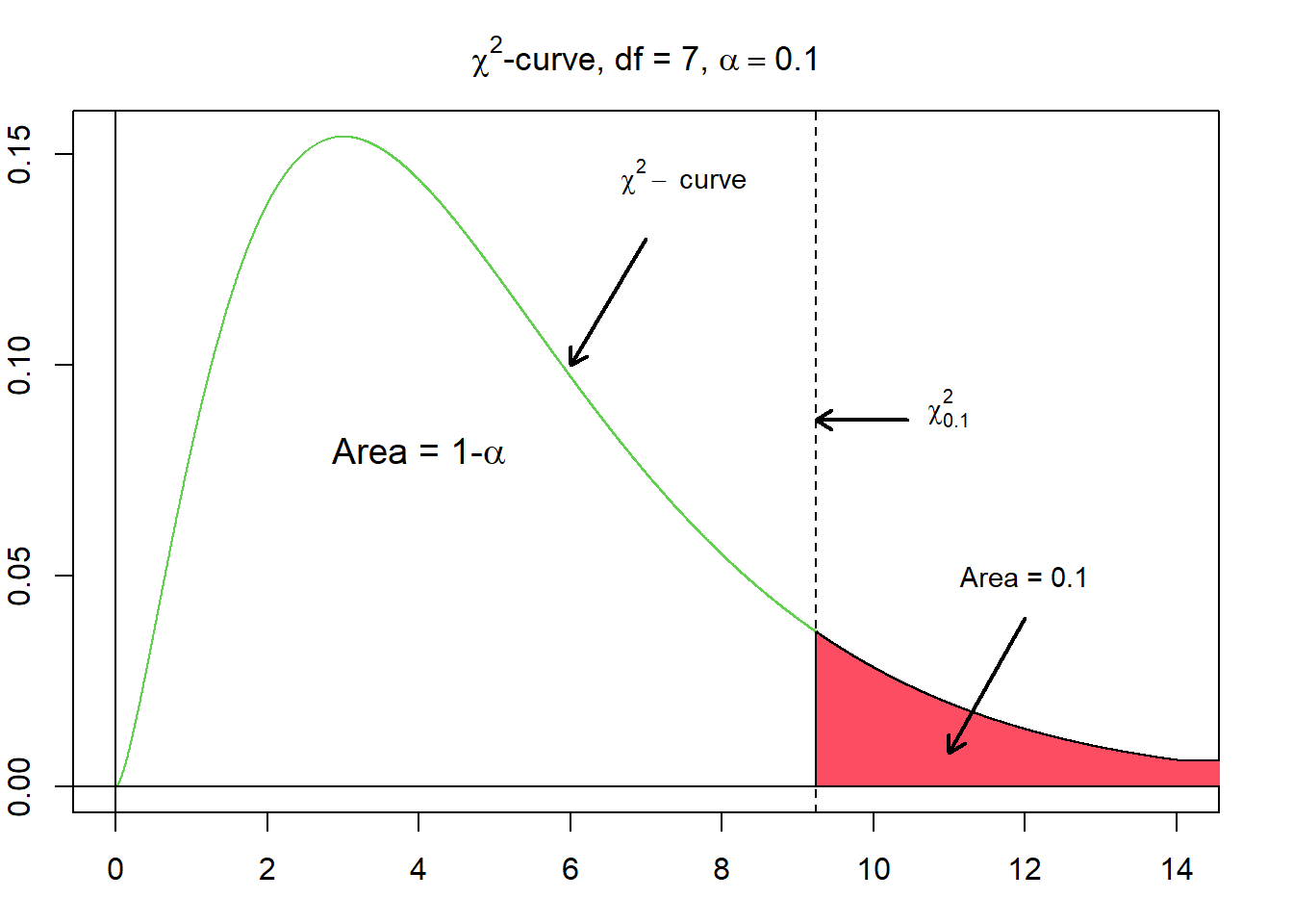
Given $\alpha$, where $\alpha$ corresponds to a probability between 0 and 1, $\chi^{2}_{\alpha}$ denotes the $\chi^{2}$-value having the area $\alpha$ to its right under a $\chi^{2}$-curve.

Interval Estimation of $\sigma$

The $100(1 − \alpha)\ \%$ confidence interval for $\sigma$ is:

$$\sqrt { \frac {n - 1} {\chi^2_{\alpha / 2}}} \le \sigma \le \sqrt { \frac{n - 1} {\chi^2_{1 - \alpha / 2}} }\text{,}$$

where $n$ is the sample size of the sample data.

One standard deviation $\chi^{2}$-test

The hypothesis testing procedure for one standard deviation is called one standard deviation $\chi^{2}$-test. Hypothesis testing for variances follows the same step-wise procedure as hypothesis tests for the mean:

---

1. State the null hypothesis $H_{0}$ and alternative hypothesis $H_{A}$.
2. Decide on the significance level, $\alpha$.
3. Compute the value of the test statistic.
4. Determine the p-value.
5. If $p \le \alpha$, reject $H_{0}$; otherwise, do not reject $H_{0}$.
6. Interpret the result of the hypothesis test.

---

The test statistic for a hypothesis test with the null hypothesis $H_{0}: \,\sigma = \sigma_{0}$ for a normally distributed variable is given by:

$$\chi^{2} = \frac {n - 1} {\sigma^{2}_{0}} s^{2} \text{.}$$

The variable follows a $\chi^{2}$-distribution with $n - 1$ degrees of freedom.

Be aware, that the one standard deviation $\chi^{2}$-test is not robust against violations of the normality assumption (Weiss, 2010).

One standard deviation $\chi^{2}$-test: An example

In order to get some hands-on experience, we apply the one standard deviation $\chi^{2}$-test in an exercise. For this, we load the students data set. You may download the students.csv file here and import it from your local file system, or you load it directly as a web resource. In either case, you import the data set to python as pandas dataframe object by using the read_csv method:

import pandas as pd
import numpy as np

students = pd.read_csv("https://userpage.fu-berlin.de/soga/data/raw-data/students.csv")

Note: Make sure the numpy, pandas and scipy packages are part of your mamba environment!

The students data set consists of 8239 rows, each representing a particular student, and 16 columns, each corresponding to a variable/feature related to that particular student. These self-explaining variables are:

• stud.id
• name
• gender
• age
• height
• weight
• religion
• nc.score
• semester
• major
• minor
• score1
• score2
• online.tutorial
• graduated
• salary

In order to showcase the one standard deviation $\chi^2$-test we examine the spread of the height in cm of female students and compare it to the spread of the height of all students (our population). We want to test, if the standard deviation of the height of female students is significantly smaller than the standard deviation of the height of all students.

Data preparation

We start with data preparation.

• Firstly, we define the standard deviation of the population. In our example the population corresponds to the height of all 8239 students in the data set. We calculate the standard deviation for the height variable and assign it the variable name sigma_0.
• Secondly, we subset the data set based on the variable gender.
• Lastly, we sample 30 female students and extract the standard deviation of the height of female students as the statistic of interest.

sigma_0 = np.std(students["height"], ddof = 1)
sigma_0

11.077529134763823

The standard deviation of the population of interest ($\sigma_{0}$) is $\approx$ 11.08 cm. Now we subset the dataset accordingly:

n = 30

female_students = students.loc[students.gender == "Female"]

female_height_sample = female_students.sample(n, random_state = 12)["height"]

sample_sd = np.std(female_height_sample, ddof = 1)
sample_sd

9.30140268744575

Further, we check the normality assumption by plotting a Q-Q plot. You can quickly generate a well-looking QQ-Plot in Python over the probplot() function provided over the stats module within the scipy package.

Note: Ensure matplotlib and scipy are installed in your mamba environment!

import matplotlib.pyplot as plt
import scipy.stats as stats

plt.figure(figsize=(12,5))
fig, ax = plt.subplots()

qq = stats.probplot(female_height_sample, dist="norm", plot = plt)
ax.set_title("Q-Q plot for weight of\n sampled female students")
ax.set_ylabel("Sample quantiles")

Text(0, 0.5, 'Sample quantiles')

<Figure size 1200x500 with 0 Axes>

As we can see, the data falls roughly onto a straight line. Based on the graphical evaluation approach we conclude, that the variable of interest is roughly normally distributed.

---

Hypothesis testing

In order to conduct the one standard deviation $\chi^{2}$-test we follow the step-wise implementation procedure for hypothesis testing.

Step 1: State the null hypothesis $H_{0}$ and alternative hypothesis $H_{A}$

The null hypothesis states, that the standard deviation of the height of female students ($\sigma$) equals the standard deviation of the population ($\sigma_{0} \approx 11.08$ cm):

$$H_{0}: \quad \sigma = \sigma_{0}$$

Alternative hypothesis:

$$H_{A}: \quad \sigma < \sigma_{0} $$

This formulation results in a left-tailed hypothesis test.

---

Step 2: Decide on the significance level, $\alpha$

$$\alpha = 0.05$$

alpha = 0.05

---

Step 3 and 4: Compute the value of the test statistic and the p-value

For illustration purposes we will manually compute the test statistic in Python. Recall the equation for the test statistic from above:

$$\chi^{2} = \frac {n - 1} {\sigma^{2}_{0}}s^{2} $$

chi_squared_value = ((n - 1) / (sigma_0**2)) * sample_sd**2
chi_squared_value

20.44603451476297

The numerical value of the test statistic is 20.4460345.

In order to calculate the p-value, we apply the chi2.cdf function derived by the scipy package over the stats module to calculate the probability of occurrence for the test statistic based on the $\chi^{2}$ distribution. To do so, we also need the degrees of freedom. Recall how to calculate the degrees of freedom:

$$df = n - 1$$

from scipy.stats import chi2

df = n - 1

p = chi2.cdf(chi_squared_value, df = df)
p

0.12147734513377556

$p = 0.121477$

---

Step 5: If $p \le \alpha$, reject $H_{0}$; otherwise, do not reject $H_{0}$

# reject H0?

p < alpha

False

The p-value is greater than the specified significance level of 0.05; we do not reject $H_{0}$.

---

Step 6: Interpret the result of the hypothesis test

At the 5 % significance level, the data provides no evidence that the standard deviation of the height of female students differs significantly from the population's standard deviation.

Hypothesis testing in Python with scipy

We just completed a one standard deviation $\chi^{2}$-test in Python manually. However, we want to implement an UDF that performs such a test based on a given dataset. Our function simple_x2_test() takes as input:

• the sample as a numpy array
• $\sigma_{0}$ as sigma_0
• $\alpha$ as alpha with 0.05 as the default value
• the test method as method with two_sided as the default value

def simple_x2_test(sample, sigma_0, alpha = 0.05, method = "two_sided"):
    
    df = sample.size - 1
    sample_std = np.std(sample, ddof = 1)
    
    chi_squared_value = (df / (sigma_0**2)) * sample_std**2
    
    if (method == "left"):
        p = 1 - chi2.cdf(chi_squared_value, df = df)
    elif (method == "right"):
        p = chi2.cdf(chi_squared_value, df = df)
    else:
        p_lower = 1 - chi2.cdf(chi_squared_value, df = df)
        p_upper = chi2.cdf(chi_squared_value, df = df)
        
        if ((p_upper * 2) > 1):
            p = p_lower * 2
        else:
            p = p_upper * 2
    
    if (p < alpha):
        reject = True
    else:
        reject = False
    
    print("Significance level: {}".format(alpha))
    print("Degrees of freedom: {}".format(df))
    print("Test statistic: {}".format(chi_squared_value))
    print("p-value: {}".format(p))
    print("Reject H0: {}".format(reject))
    
    return reject

Let us apply our self-built function simple_x2_test() to the example data from above.

simple_x2_test(female_height_sample, 11.08, 0.05, "right")

Significance level: 0.05
Degrees of freedom: 29
Test statistic: 20.436916507013866
p-value: 0.12117213234555052
Reject H0: False

False

Perfect!

---

Citation

The E-Learning project SOGA-Py was developed at the Department of Earth Sciences by Annette Rudolph, Joachim Krois and Kai Hartmann. You can reach us via mail by soga[at]zedat.fu-berlin.de.

You may use this project freely under the Creative Commons Attribution-ShareAlike 4.0 International License.

Please cite as follow: Rudolph, A., Krois, J., Hartmann, K. (2023): Statistics and Geodata Analysis using Python (SOGA-Py). Department of Earth Sciences, Freie Universitaet Berlin.