In order to decide whether to reject the null hypothesis, a test statistic is calculated. The decision is made based on the numerical value of that test statistic. There are two approaches how to arrive at that decision:
By applying the critical value approach, it is determined whether or not the observed test statistic is more extreme than a defined critical value. Therefore, the observed test statistic (calculated based on sample data) is compared to the critical value (a kind of cutoff value). The null hypothesis is rejected if the test statistic is more extreme than the critical value. The null hypothesis is not rejected if the test statistic is not as extreme as the critical value. The critical value is computed based on the given significance level $\alpha$ and the type of probability distribution of the idealized model. The critical value divides the area under the probability distribution curve in rejection region(s) and non-rejection region.
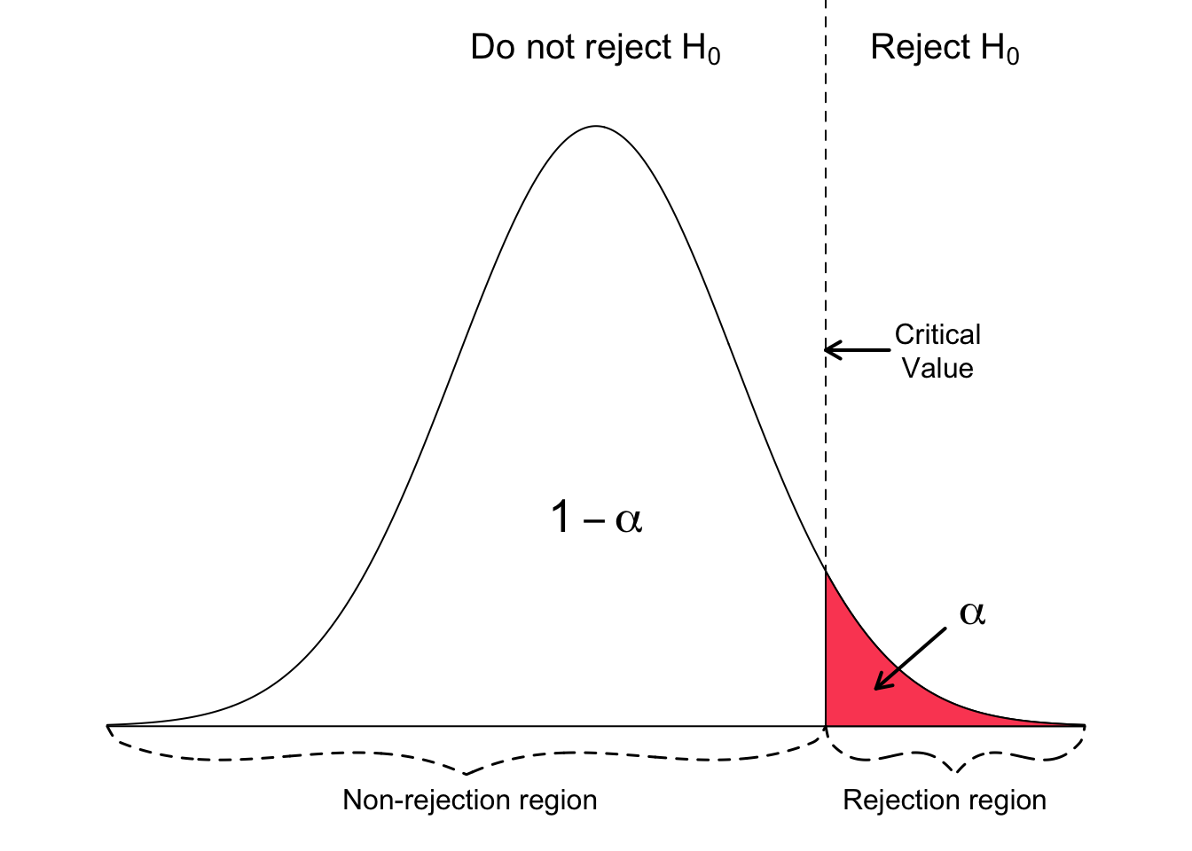
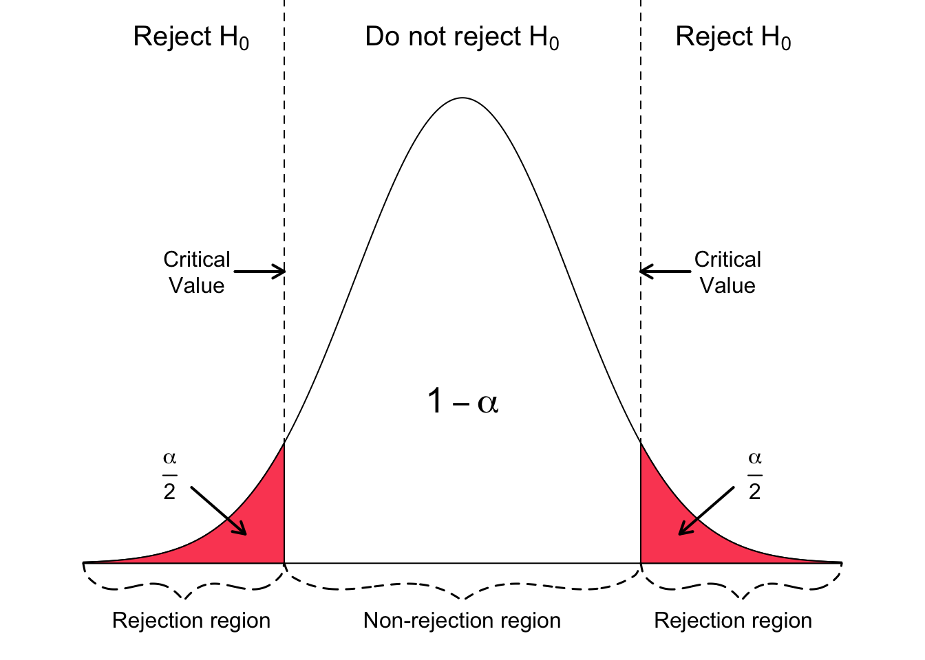
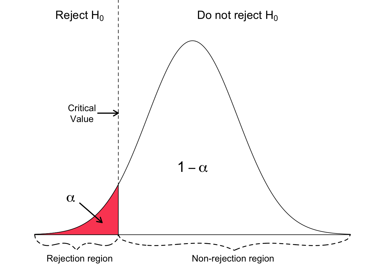
The following three figures show a right-tailed, left-tailed, and two-sided test. The idealized model in the figures, and thus $H_{0}$, is described by a bell-shaped normal distribution curve.
In a two-sided test, the null hypothesis is rejected if the test statistic is too small or too large. Thus, the rejection region for such a test consists of two parts: one on the left and one on the right.
The null hypothesis is rejected for a left-tailed test if the test statistic is too small. Thus, the rejection region for such a test consists of one part left from the centre.
The null hypothesis is rejected for a right-tailed test if the test statistic is too large. Thus, the rejection region for such a test consists of one part right from the centre.
For the p-value approach*, the likelihood (p*-value) of the numerical value of the test statistic is compared to the specified significance level ($\alpha$) of the hypothesis test.
The p-value corresponds to the probability of observing sample data at least as extreme as the actually obtained test statistic. Small p-values provide evidence against the null hypothesis. The smaller (closer to 0) the p-value, the stronger is the evidence against the null hypothesis.
The null hypothesis is rejected if the p-value is less than or equal to the specified significance level $\alpha$. Otherwise, the null hypothesis is not rejected.
Note: if $p \le \alpha$, reject $H_{0}$; otherwise, if $p > \alpha$, do not reject $H_{0}$.
Consequently, by knowing the p-value, any desired significance level may be assessed. For example, if the p-value of a hypothesis test is 0.01, the null hypothesis can be rejected at any significance level larger than or equal to 0.01. It is not rejected at any significance level smaller than 0.01. Thus, the p-value is commonly used to evaluate the strength of the evidence against the null hypothesis without reference to the significance level.
The following table provides guidelines for using the p-value to assess the evidence against the null hypothesis (Weiss, 2011):
p-value | Evidence against $H_{0}$ |
---|---|
$$p > 0.10$$ | Weak or no evidence |
$$0.05 < p \le 0.10$$ | Moderate evidence |
$$0.01 < p \le 0.05$$ | Strong evidence |
$$p \le 0.01$$ | Very strong evidence |
Citation
The E-Learning project SOGA-Py was developed at the Department of Earth Sciences by Annette Rudolph, Joachim Krois and Kai Hartmann. You can reach us via mail by soga[at]zedat.fu-berlin.de.
Please cite as follow: Rudolph, A., Krois, J., Hartmann, K. (2023): Statistics and Geodata Analysis using Python (SOGA-Py). Department of Earth Sciences, Freie Universitaet Berlin.