Introduction to JupyterLab

If you do not intend to use JupyterLab through your SOGA experience, please feel free to skip this chapter.

In the following guide the most important features of JupyterLab for the purposes of this tutorial will be introduced, as we recommend the use of JupyterLab as IDE for your journey through this Python tutorial. Firstly, the basic concepts of the Jupyter environment will be explained, followed by elaborating on the usage of JupyterLab with a focus on the possibility of combining code with markdown structured text in Jupyter notebooks.

This guide is intended as a brief introduction guide to get you familiar with JupyterLab in general. Please feel free to have a look on the great online documentation of JupyterLab.

General Concepts

The key element of JupyterLabs IDE is Jupyter Notebook files. These Notebooks enable the user to combine code that is directly executable, and can be wrapped in narrative text. This narrative text is written in a markdown structure which is similar to Latex. Overall by using Jupyter Notebooks you can combine the following content types in one compact, well-structured and optically pleasing file:

• Live-code
• Interactive widgets
• Plots
• Narrative text
• Equations
• Images
• Video

For these purposes, the JupyterLab IDE consists of three main components:

• The notebook web application: An interactive web application for authoring notebook documents, writing and running code interactively.
• Kernels: Separate processes started by the notebook web application that runs users' code in a given language and returns output back to the notebook web application. The kernel also manages things like computations for interactive widgets, tab completion and introspection.
• Notebook documents: Self-contained documents that contain a representation of all content visible in the notebook web application. This includes inputs and outputs of the computations, narrative text, equations, images, and rich media representations of objects. Each notebook document has its own kernel.

Note: By default, the kernel runs Python code. Nevertheless, you can easily change the kernel to other supported programming languages. In this way you can use Jupyter Notebooks also in combination with R for instance. Please refer to Jupyters online documentation for more information.

JupyterLab in Action

To start the JupyterLab IDE from your mamba environment, just activate your personal environment with JupyterLab installed and use the following command:

jupyter lab

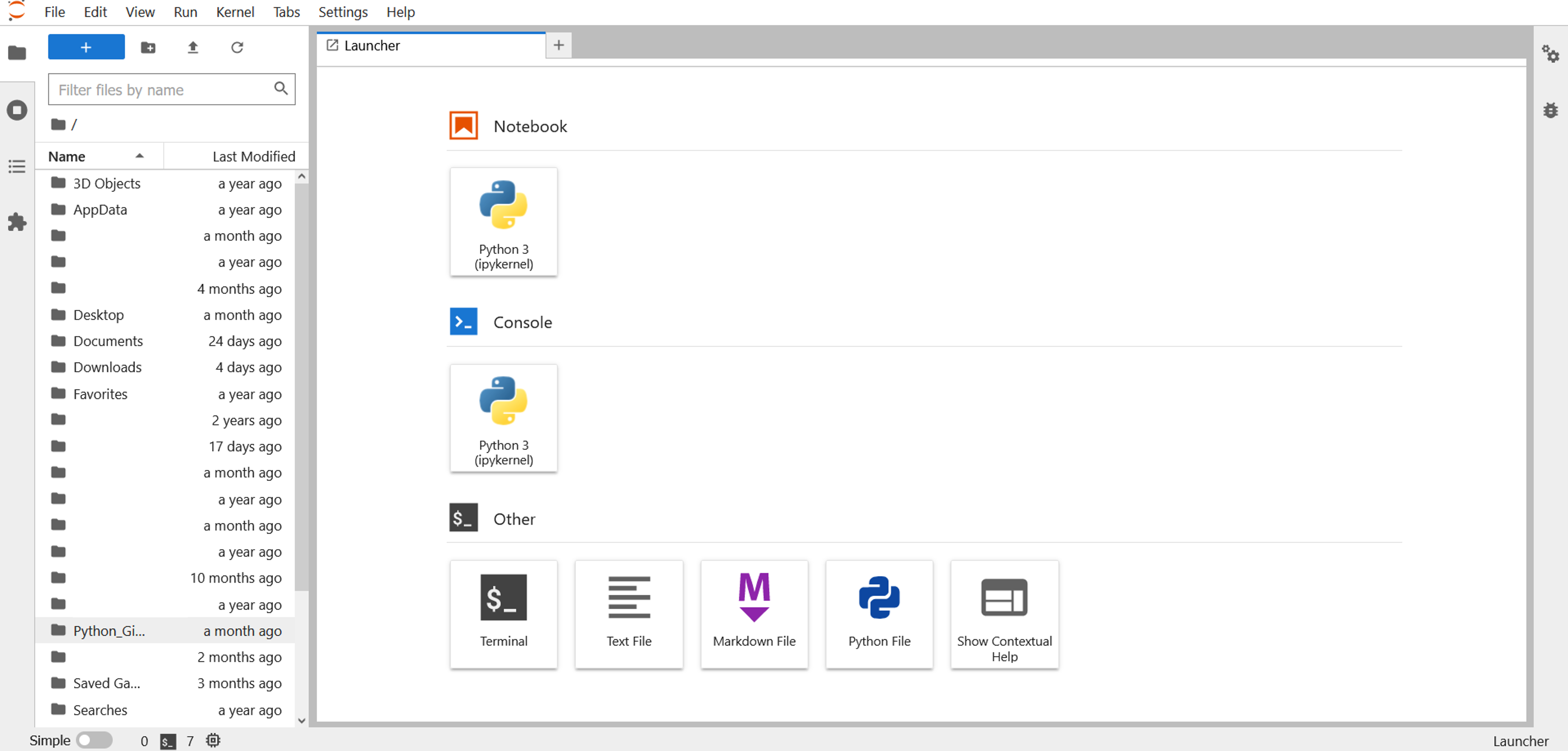
This will start a local webserver in your mamba environment. At the same time, the JupyterLab dashboard is displayed in your default browser. If JupyterLab is started for the first time, the dashboard should look like this:

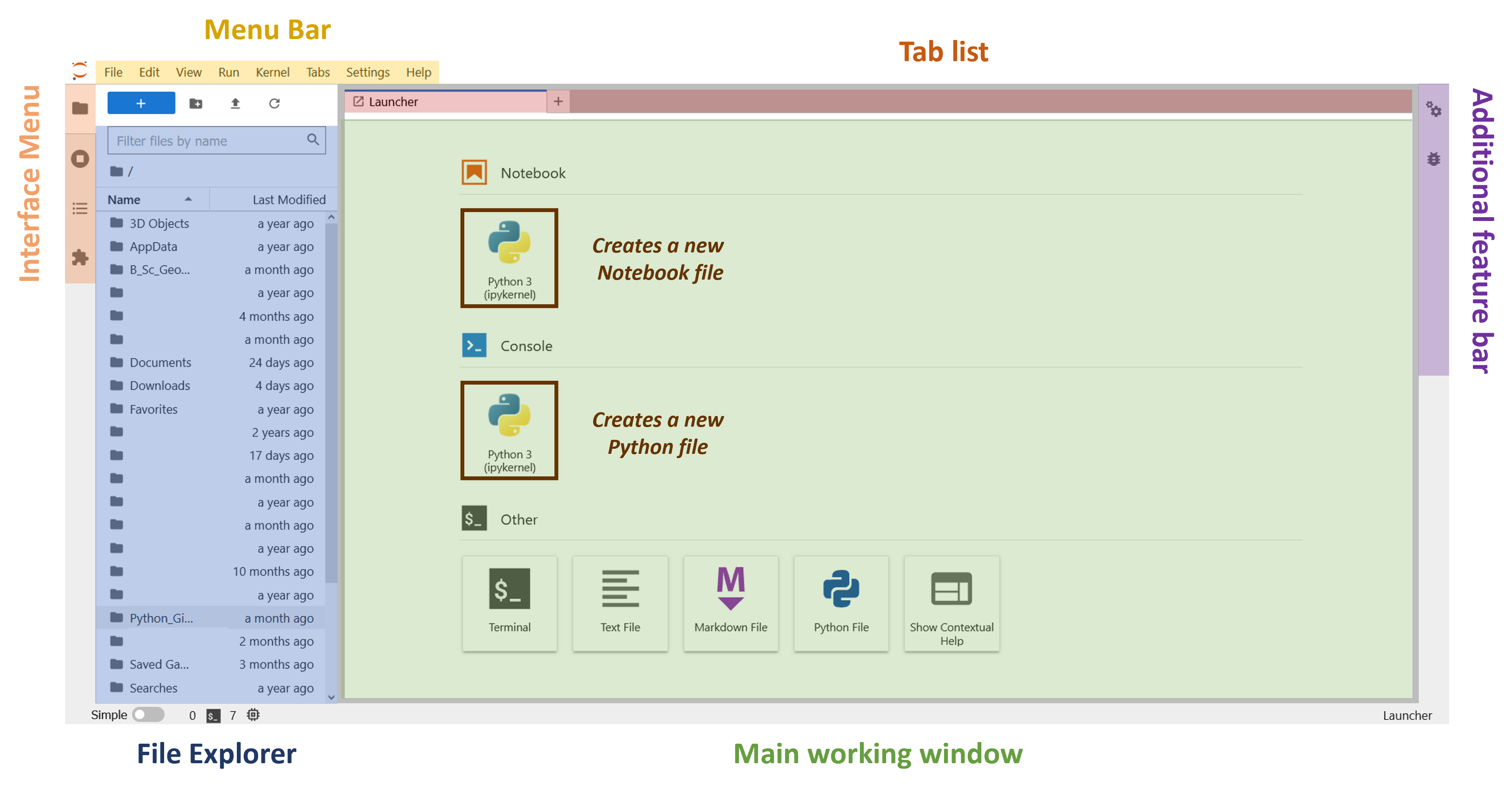
An Overview of the most important features that you can find over this dashboard is given in the following illustration.

Note: The notebook server will be started at the file system location where you run the above command in your command line interface. It is reasonable to switch your working directory manually over the command line to a different location. Start the notebook server afterwards. Make sure that the directories that you are looking for are listed and accessible over the file explorer window in JupyerLab.

Working with Jupyter Notebooks

Creation of a new Notebook file

To create a new notebook file, just click on the icon creates a new notebook file, as shown in the above illustration, where the icon is surrounded by a brown border. This will create a new blank Python notebook file at the location of your actual working directory.

In your working window a new Python notebook is added:

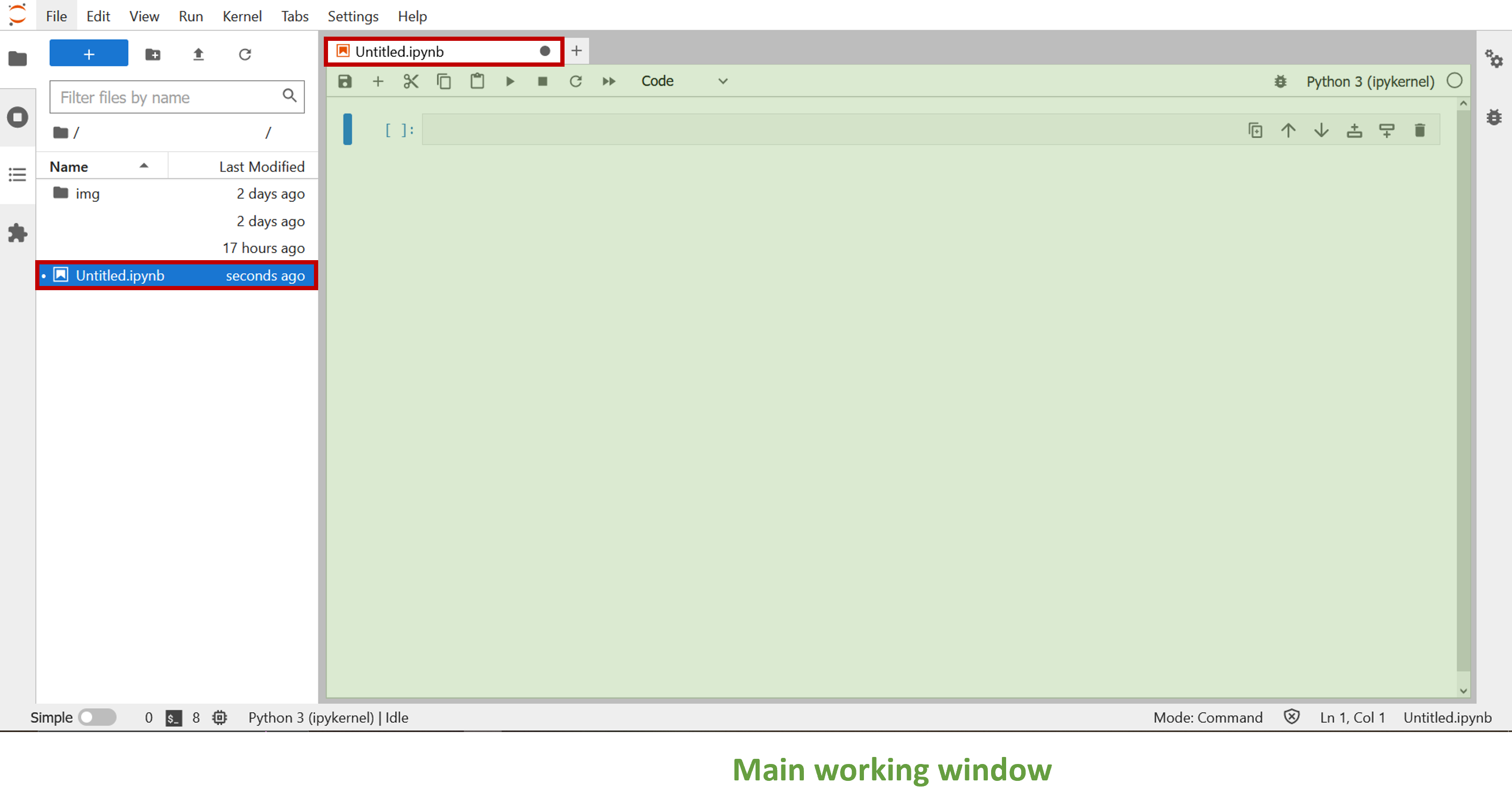
Note: Jupyter Notebook files are saved to disk with the suffix .ipynb. You can only edit and display these files properly within a Jupyter IDE comparable to word or excel files.

In addition, you find the fast feature access bar, integrated in your new created notebook, inside the main working window:

A summary of the meanings of the features is given below.

Toolbar Symbol	Meaning
	Save current notebook file
	Add a new cell to the current notebook
	Cut one or more selected cells
	Copy one or more selected cells
	Paste cells from clipboard into the current notebook file
	Execute one or more selected cells
	Stop execution
	Restart kernel
	Restart kernel and run all cells of the current notebook file
	Change cell type

Notebook cells

In Jupyter Notebooks it is all about cells. You can use these cells to either write live executable code fragments or to display formattable text passages. This text could also contain images, videos, equations or whatever you like to add to your narrative text. As you can also insert direct html statements, there are no bounds for your creativity. But one after another. If you have a closer look to your newly created notebook, you will see that a first blank output cell is already added to your notebook by creation:

Every notebook cell consists of three main components:

• An indication wether this cell in executable
• the cell content
• a cell specific tool bar

Notebook cell types

As mentioned above you can choose between different cell types in Jupyter Notebooks according to your content type. The different cell types are:

1. Code cells: These cell types allow you to write and run code snippets interactively. They were executed asynchronously. Every new cell in a notebook file is created as code cell by default.
2. Markdown cells: These cells are used to add narrative text of any kind to your notebook file. As stated before you can also add equations, images, videos or other contents to these cells. The text formatting and content bindings are interpreted over the markdown markup language. An Overview of the options that exist inside these cells is given in Jupyters online documentation about markdown cells.
3. Raw cells: These cells are not interpreted in any way. You could use these for instance to share code snippets that should not be executable or in general for any information that should not be interpreted and rendered by the computer. Hence the cell content will be display originally as you wrote it in this cell.

Change cell type

If you click on a cell inside of a Jupyter Notebook the notebooks toolbar will show you the specific cell type. For example, the cell in the following screenshot is a code cell:

You can change the type of one or more selected cells by clicking on the little arrow besides the cell type. This will open a context menu which lists the cell types described above:

You can also use keyboard shortcuts to change the cell type

• c == change selected cell to coding cell
• m == change selected cell to markdown cell
• r == change selected cell to raw cell

Execution of code

To run a code snippet inside of a code cell just select the desired notebook cell and click on the button in the notebook's toolbar. Alternatively you could use the keyboard shortcut shift + enter.

print("Hello, you just executed this cell")

Summary

What you just learned is everything you need to know to start your own experience using Jupyter Lab. Please feel free to have a look on the online documentation of Jupyter Lab, where all features are explained in detail very nicely. Furthermore, you can find YouTube videos in which the usage of JupyterLab is presented. Below, you can find a list of the most important key board shortcuts to make your start with Jupyter Lab easier. We hope you enjoy your work with JupyterLab!

Keyboard Short Cut	Meaning
up	Navigates upwards to the next cell in your notebook file
down	Navigates downwards to the next cell in your notebook file
s	Save the notebook file to disk
a	Inserts a new cell above the selected cell
b	Inserts a new cell below the selected cell
c	Copies selected cells to clipboard
v	Inserts the copied cells from clipboard
x	Copies selected cells to clipboards and deletes them at the same time
dd	Deletes selected cells. Needs to be tipped doubled due to pretend you from accidentally deletes
shift + enter	Executes the selected cells

---

Citation

The E-Learning project SOGA-Py was developed at the Department of Earth Sciences by Annette Rudolph, Joachim Krois and Kai Hartmann. You can reach us via mail by soga[at]zedat.fu-berlin.de.

You may use this project freely under the Creative Commons Attribution-ShareAlike 4.0 International License.

Please cite as follow: Rudolph, A., Krois, J., Hartmann, K. (2023): Statistics and Geodata Analysis using Python (SOGA-Py). Department of Earth Sciences, Freie Universitaet Berlin.